
Attachment 'thesis.tex'
Download 1 \documentclass[letterpaper,12pt,oneside]{book}
2 \usepackage{geometry} % to change the page dimensions
3 \geometry{margin=1.25in} % for example, change the margins to 2 inches all round
4 \usepackage[style=numeric-comp,backend=bibtex]{biblatex}
5 % bibtool -s -d refs.bib muyuan_all.bib ludtke_lab.bib -o references.bib
6 % \addbibresource{refs.bib}
7 % \addbibresource{mendeley.bib}
8 \addbibresource{paperpile.bib}
9 % \addbibresource{ludtke_lab.bib}
10 % \addbibresource{muyuan_all.bib}
11 % \addbibresource{mapchallenge.bib}
12 % \addbibresource{references.bib}
13 \usepackage{float}
14 \usepackage{setspace}
15 \doublespacing% Double-spaced document text
16
17 \usepackage{ccaption}
18 \usepackage{caption}
19 % \DeclareCaptionJustification{double}{\doublespacing}
20 % \captionsetup[figure]{labelfont=bf,font=doublespacing,justification=double}
21 % \captionsetup{font=doublespacing}% Double-spaced float captions
22
23 \usepackage{rotating}
24
25 \usepackage{amsmath}
26 \usepackage{amsfonts}
27 \usepackage{amssymb}
28
29 \usepackage{fontspec}
30 \usepackage{titlesec}
31
32 \setmainfont{Times New Roman}
33 \setsansfont{Times New Roman}
34
35 \titleformat{\section}
36 {\normalfont\fontsize{16}{15}\bfseries}
37 {\thesection}
38 {1em}
39 {}
40 \titlelabel{\thetitle.\quad}
41
42 \titleformat{\subsection}
43 {\normalfont\fontsize{14}{15}\bfseries}
44 {\thesection}
45 {1em}
46 {}
47 \titlelabel{\thetitle.\quad}
48
49 \titleformat{\subsubsection}
50 {\normalfont\fontsize{14}{15}\bfseries}
51 {\thesection}
52 {1em}
53 {}
54 \titlelabel{\thetitle.\quad}
55
56 \usepackage{graphicx} % support the \centering \includegraphics command and options
57 \graphicspath{{figures/}} % Directory in which figures are stored
58 \usepackage{afterpage}
59 \usepackage{fancyhdr}
60 \usepackage{microtype}
61 \usepackage{pdfpages}
62 \newcommand{\angstrom}{\textup{\AA}}
63 \fancyhf{}
64 \renewcommand{\headrulewidth}{0pt}
65 %\raggedright
66 \righthyphenmin 6
67 \lefthyphenmin 5
68 %\hyphenpenalty 8000
69 %\exhyphenpenalty 10000
70 % \renewcommand{\familydefault}{\sfdefault}
71
72 \usepackage{hyperref}
73 \hypersetup{colorlinks=false}
74
75 \setcounter{tocdepth}{5}
76 % \setcounter{secnumdepth}{5}
77
78 \newcommand{\nocontentsline}[3]{}
79 \newcommand{\tocless}[2]{\bgroup\let\addcontentsline=\nocontentsline#1{#2}\egroup}
80
81 \cfoot{\thepage}
82 \pagestyle{fancy}
83
84 \title{COMPUTATIONAL WORKFLOWS FOR ELECTRON CRYOMICROSCOPY \\
85 \vspace{1cm}
86 \normalsize
87 A Dissertation Submitted to the Faculty of \\
88 The Graduate School\\
89 Baylor College of Medicine \\
90 \vspace{1cm}
91 In Partial Fulfillment of the\\
92 Requirements for the Degree \\
93 of\\
94 Doctor of Philosophy\\
95 by\\
96 }
97 \author{JAMES MICHAEL BELL}
98 \date{
99 Houston, Texas\\
100 March 21, 2019
101 }
102
103 \begin{document}
104
105 \setcounter{page}{1}
106 % \addcontentsline{toc}{chapter}{Title}
107 \maketitle
108 \clearpage
109
110 \setcounter{page}{2}
111 \addcontentsline{toc}{chapter}{Approvals}
112 \includepdf[pages={1}]{sign_page.pdf}
113
114 \setcounter{page}{3}
115 \chapter*{Acknowledgment}
116 \addcontentsline{toc}{chapter}{Acknowledgment}
117
118 I have benefited greatly from the support of others throughout graduate school. There are so many individuals that provided academic and moral support as I completed the research described in this thesis, and I feel compelled to acknowledge and thank a number of them here.
119
120 I'd like to begin by thanking my doctoral advisor, Steve Ludtke for his academic and professional guidance and financial support as I pursued my doctoral degree. It was a privilege to receive mentorship from an individual with such a deep grasp of physics and computing and strong ties to the cryoEM community. Graduate school was my first exposure to working as a member of a large organization, and Steve’s insights were exceptionally valuable as I learned and grew in this new environment. Likewise, Steve taught me not only about scientific concepts but also how science works in practice. I appreciate the autonomy he provided as I explored research directions and careers as well as the guidance he provided when solicited. I have also enjoyed learning from Steve about a broad range of topics from 3D printing and imaging physics to cluster administration and navigating the corporate world.
121
122 Next, I'd like to thank the members of my thesis advisory committee, Mike Schmid, Henry Pownall, Irina Serysheva, Ming Zhou, and Zhao Wang, for their guidance, support, and advice. Mike was one of the best teachers under whom I have had the pleasure to study. He is truly a master of the Socratic method, and I enjoyed working with him on a range of projects from electron cryotomography to nanocrystal indexing. I am honored that he has remained a part of my thesis advisory committee after moving to Stanford. Henry has provided lots of outstanding scientific and life advice, and I have appreciated his willingness to share these insights alongside biological samples for research. I am thankful also to the members of Henry’s lab, namely Baiba Gillard, Dedipya Yelamanchili, and Bingqing Xu, for helping procure high-density lipoprotein samples for imaging. Irina has been consistently encouraging, and I have appreciated her generosity in allowing me to use some of her group's electron microscopes for imaging projects. Ming has been an incredible committee member and has always made me feel like a close colleague. His excellent questions at each of my committee meetings helped me evaluate and enhance my research. Finally, Zhao and I share a lot of excitement about new ideas in the field of cryoEM. In addition to appreciating his participation on my committee, I am thankful for his including me in discussions about some of his lab’s research. I am also thankful for the use of imaging data recorded by members of his lab, particularly Zhili Yu and Xiaodong Shi, to test the EMAN2 tomography workflow.
123
124 When I joined the Ludtke lab, I was surrounded by highly-experienced individuals who really helped catapult my research forward. Jesus Galaz Montoya taught me about electron cryo-tomography and was instrumental in me passing my qualifying exam. Also, Stephen Murray introduced me to Henry Pownall and helped me locate literary resources on high-density lipoprotein, which guided a significant fraction of my doctoral research. Since joining, I have worked closely with Adam Fluty and Muyuan Chen, who have been incredible, generous colleagues. Over the past few years, Adam has provided lots of useful cellular tomography data for testing purposes, and I have really enjoyed our discussions on a wide variety of topics. Muyuan has played a tremendous supporting role in my graduate career, and I am so thankful for our discussions and collaboration. Our conversations have offered great insight into science and machine learning concepts, and I have grown rather fond of his sense humor. I wish each of these individuals the best as they take the next steps in their careers.
125
126 Beyond the Ludtke lab, I feel compelled to mention my appreciation for members of the National Center for Macromolecular Imaging (NCMI) with whom I worked extensively throughout the majority of my graduate studies. Many of my research projects started after conversations with Wah Chiu, the director of the NCMI. Wah involved me in a range of projects including participating in the EMDatabank Map Challenge community validation effort, which produced a number of spin-off projects discussed in this thesis. I am also appreciative of conversations and collaborations with David Chmielewski, Boxue Ma, Zhaoming Zu, and Kaiming Zhang, and Jason Kaelber, each of whom provided imaging data, support, and scientific insights.
127
128 I feel lucky to have been guided not only by my work colleagues but also by many of my teachers. Two, in particular, stand out at the end of my graduate studies, namely Ted Wensel, and Devika Subramaniam. Besides expanding my biological and computational knowledge base, these individuals largely shaped the direction of my graduate research and ultimately my chosen career direction. Ted taught a class on molecular biophysics, which helped me establish a useful and intuitive frame of reference for the biological subjects I was examining, many of which I was learning about for the first time. It was the perfect framing of biological and molecular methods for someone with a physics degree but considerably less exposure to the biological sciences. Devika taught a course on statistical machine learning, which was without a doubt the most impactful class I have ever taken. At the time I took the course, I was amazed by her unique and intuitive manner of conveying complex material; however, even after the course, I was unaware of just how applicable and marketable the content I learned would be. Now, as I take the next step toward a career in data science, I recognize that my awareness of this field and the latest methods in machine learning are largely due to Devika’s paradigm-shifting lectures and class projects.
129
130 Next, I’d like to acknowledge my mentors both old and new that have helped shape me into the person I am today. These include Brett Matherne, Shadow Robinson, Angela Wilkins, and David Dilger. Brett has always been a great sounding board since I was in high school, and I always appreciated how he took me seriously (but not too seriously). Shadow instilled a passion for science in me and helped enhance my graduate applications and studies through his encouragement to pursue an international research experience for undergraduates (IREU). It has been inspiting to work with Angela to create data science solutions for businesses, and I truly appreciate her guidance as I transition from academia to industry. Lastly, it has been a pleasure getting to know David. His professional advice and words of affirmation have offered an incredible confidence boost. I am honored to call him a mentor and a friend. I am so thankful for the influence these individuals have had and will continue to have on my life in the years to come.
131
132 Through graduate school, I have met so many new friends. Four of which were there from day one, and I want them to know how much I have appreciated our friendship. To Danny Konecki, Chih-Hsu Lin, Pei-Wen Hu, and Justin Mower: cheers, guys! Danny, you are incredibly smart, and your compassion for others never ceases to amaze me. I can’t wait to see what you do next! Chih-Hsu and Pei-Wen, I am so thankful for the time we have spent together as Chih-Hsu and I have pursued the same degree. I am also honored to have been granted the title “Uncle Michael” and will continue to enjoy watching Amelia grows up. But she really needs to slow down! Justin, thank you for all of the fun, insightful conversations, and best of luck as you continue in your professional pursuits. Perhaps we will get to work together again someday! Beyond these individuals, I am thankful for my friendships with Stephen Wilson, Jonathan Gallion, and Nick Abel who have been part of some of the most fun and memorable experiences of my graduate career.
133
134 As I approach the end of my rather long list of acknowledgments, I want to express my love and deepest gratitude to a group who I cannot possibly offer sufficient thanks: my family.
135
136 To my parents, Beth and Marlon, thank you for your support through the ups and downs and for encouraging me to stay the course when I did not think I had it in me. To my grandparents, Jim, Jayne, and Betty, thank you for your encouragement and your optimism about what lies ahead. To my sister and her fiance, Emily and Edward: thank you for your encouragement, and best wishes to both of you as you begin your married life together later this year. To my uncle, Stephan, thank you for demonstrating to so many the power and reach of one's hard work and dedication. To my aunt and cousin, Michelle and Christopher, thanks for your support and comic relief, from spider-man tissues to tortas. To my in-laws, Douglas and Leigh: thank you for believing in me and listening intently since met you during my first visit to Starkville. To my two cats, Holly and Frida: thank you for putting a smile on my face every time I walk through the door. And finally, to my wife, Claire: Thank you for your patience, your compassion, your strength, your foresight, and your courage. I love you. Now it’s your turn to graduate.
137
138 In addition to the individuals mentioned above, I am thankful for the support and funding I received from the Gulf Coast Consortia through a Houston Area Molecular Biophysics Program training grant (T32GM008280). Additionally, I greatly appreciate the research funding provided by the NIH through a variety of grants that have allowed me to participate in cryoEM research (R01GM080139, R01GM079429, P41GM103832). Finally, I'd like to acknowledge and thank the directors and administrators of the Quantitative and Computational Biosciences graduate program and the Verna and Marrs McLean Department of Biochemistry and Molecular Biology at Baylor College of Medicine for their guidance and encouragement along the way.
139
140 \chapter*{Abstract}
141 \addcontentsline{toc}{chapter}{Abstract}
142
143 Electron cryomicroscopy (cryoEM) is widely used for the near-native structure determination of macromolecular complexes. CryoEM data collection begins with sample vitrification to lock specimens in near-native conformations prior to imaging via transmission electron microscopy (TEM). Specimen images are then extracted from raw micrographs and used to generate a 3D reconstruction through a workflow called single particle analysis (SPA) . Using this technique it is possible to obtain 3D structures at resolutions higher than 8$\angstrom$, with some achieving crystallographic resolutions better than 2$\angstrom$.
144
145 Alternatively, if the specimen is tilted during image acquisition through a procedure known as electron cryo-tomography (cryoET), the tilted micrographs can be combined computationally to produce a large 3D representations of the bulk sample. Sub-volumes can be extracted from these 3D reconstructions, aligned to a reference model, and averaged via a workflow known as subtomogram averaging to yield protein structures, occasionally at resolutions higher than 10$\angstrom$.
146
147 Modern cryoEM experiments generate massive amounts of data, requiring tremendous effort to process toward new biological conclusions; however, the gradual development and automation of computational workflows in user-friendly software packages continues to reduce this burden. One such package, EMAN2, offers complete workflows for the 3D reconstruction of cryoEM data.
148
149 In this thesis, I describe my contributions to EMAN2 that expedite data processing and enhance structural resolutions.
150
151 Chapter 1 provides an overview of structural biology, cryoEM data collection, and computational workflows for cryoEM image processing. This chapter targets non-experts interested in cryoEM, seeking to provide intuition and definitions in preparation for more advanced topics discussed in later chapters.
152
153 In chapter 2, I present unpublished research on global and local corrections for specimen motion, corresponding to the first stage of image processing in cryoEM. Here, I compare motion correction algorithms and examine the influence of measured trajectory discrepancies. I also analyze the influence of motion correction algorithms on resolution and discuss a novel use of trajectory information for bad micrograph identification and removal.
154
155 In chapter 3, I explore the high-resolution SPA pipeline in EMAN2 and discuss the philosophy behind the methods we use to approach to the 3D reconstruction problem. I also present some of my benchmarking results, demonstrating the performance of EMAN2 prior to the work outlined in the following chapter.
156
157 In chapter 4, I outline new software tools for the EMAN2 SPA workflow that were inspired by my findings during the 2015 EMDatabank Map Challenge. I detail my collaborative work in the development and implementation of a new strategy for particle picking, a new particle quality metric, and alterations in the global and local filtration of 3D reconstructions. These changes improve automation and dramatically improve the appearance of side-chains in high-resolution structures.
158
159 In chapter 5, I describe collaborative work resulting in a complete, integrated workflow for cryoET and subtomogram averaging in EMAN2 that is capable of achieving state-of-the-art resolutions in purified and cellular datasets. My role in this research was to integrate numerous workflow components, develop graphical user interfaces, and arrange for consistent metadata handling throughout the workflow. These contributions greatly reduce human effort and increase the throughput of cryoET data processing.
160
161 Finally, in chapter 6, I discuss my perspectives about the future of cryoEM as it relates to my research. Additionally, in an appendix I discuss unpublished cryoEM experiments in which I resolve the structure of nascent high-density lipoprotein to roughly 50$\angstrom$ through subtomogram averaging.
162
163 Looking ahead, further optimization of computational workflows for cryoEM will offer increasingly direct paths toward structure determination and biological insights. As more structures are determined, we will continue to enhance our understanding of the macromolecular machinery that enables life at the cellular level.
164
165 \tableofcontents
166 \listoffigures
167 \listoftables
168
169 \chapter{Introduction}
170
171 This chapter targets non-experts interested in electron cryo-microscopy (cryoEM), seeking to provide intuition and definitions in preparation for more advanced topics discussed in later chapters. I begin with an overview of structural biology and various methods for obtaining structural information about biological macro-molecules, with particular emphasis on cryoEM. Next, I describe cryoEM data collection and some of the recent technological developments that have dramatically improved the quality of cryoEM structures. Finally, I outline three key image processing workflows in cryoEM that are enhanced and further automated by my doctoral research.
172
173 \newpage
174
175 \section{What is structural biology?}
176
177 When you think of a simple mechanical system, it is almost immediately apparent what it is designed to do. For example, consider a tricycle. In the simplest case, a tricycle consists of a solid frame, a seat, two round wheels at the rear, handlebars, and pedals connected to a large front wheel, all of which are necessary for a tricycle to move forward under forces applied by a rider. Now consider what might happen if any of these components were removed. The bicycle would no longer function properly, and our assumptions about how it behaves would no longer be valid. Without handlebars, it would be impossible to maneuver. Without wheels or pedals, the tricycle would not move forward.
178
179 While this conceptualization ignores many of the inherent complexities of the individual components, it offers insight into the important relationship between an object’s structure and its function. We do not need to fully understand the dynamics of a moving bicycle to gain valuable functional insight from its structure alone. This same structure-function paradigm has guided research in the field of structural biology since its conception; however, instead of studying the relatively intuitive relationships between the morphology of macroscopic objects and their function, structural biologists are interested in determining the structures and molecular organization of individual proteins and macromolecular complexes and drawing inference from them to answer pressing biological questions.
180
181 The functional mechanisms of individual proteins and their biological roles within the context of cells are significantly more complex than the tricycle example above. When biologists talk about a protein, they are referring to an organic, polymer chain formed by a sequence of amino acid residues with one or more biological functions. There are 22 unique amino acid residues that are used to construct proteins, each of which has unique physicochemical properties that govern how proteins fold in 3D and interact with other molecules. While some proteins are intrinsically disordered and do not fold into a consistent 3D structure under physiological conditions, many proteins naturally fold into conformations that enable their highly-specialized protein functions, and others require the mediation of other proteins to fold into their functional state.
182
183 Certain classes of proteins perform relatively intuitive functions. For example, protein complexes called ribosomes are responsible for manufacturing other proteins by translating the information encoded in ribonucleic acid (RNA) into proteins (Figure \ref{fig_structbio} A1). Membrane pumps move substances across the cellular membrane to maintain homeostatic conditions by modulating the concentration of ions and other molecules inside cells (Figure \ref{fig_structbio} A2). Enzymes are another common type of protein that catalyze chemical reactions so they occur fast enough to sustain key cellular functions (Figure \ref{fig_structbio} A3). In light of these descriptions, it is clear that the cell is a factory for macromolecular machines, and the structure-function paradigm tells us that understanding the structural details of these components will grant insight into how these proteins interact and function in the crowded cellular environment to facilitate life.
184
185 Despite their small size (with diameters ranging from 0.4-100$\mu$m), individual cells correspond to profoundly intricate systems with an immense number of molecules that enable cellular function and reproduction. Simple calculations reveal that individual cells contain millions of proteins \cite{Milo2013-ye}. The field of structural biology exists to obtain a better understanding the structures and functions of each of these machines, generally focusing on features ranging from the placement of individual atoms to the organization of large macromolecular complexes. These diverse features occur at scales from angstroms to a hundreds of nanometers, though structural biologists do occasionally study features with lengths of multiple microns when examining macromolecular complexes within whole cells (Figure \ref{fig_structbio} B).
186
187 Structural biology describes the various levels of protein organization in a hierarchy consisting of primary, secondary, tertiary, and quaternary structural elements (Figure \ref{fig_structbio} C). When studying any protein, it is important to consider interactions that occur within each of these categories. For example, knowledge of a protein’s primary structure, also called its sequence, enables us to identify other proteins with similar sequences that often have similar functional roles. Secondary and tertiary structure elements offer important 3D information that tell us about interaction sites and can be leveraged for rational drug design. At the highest level, quaternary structure tells us about how multiple protein chains bind together, and is particularly important when examining complexes that consist of more than one subunit. The information encoded in each of a protein’s structural elements provides insight into its functional role and how it may interact with nearby proteins and protein complexes.
188
189 \afterpage{
190 \begin{figure}[p]
191 \centering \includegraphics[width=.9\linewidth]{fig_structbio}
192 \vspace{1cm}
193 \caption[Overview of structural biology]
194 {Overview of structural biology${}^{*}$ (Continued on next page).
195 \footnotesize \newline \newline $*$Protein illustrations in A and B are licensed under a \href{https://creativecommons.org/}{Creative Commons} \href{creativecommons.org/licenses/by/4.0/legalcode}{Attribution 4.0 International} license by David S. Goodsell and the RCSB PDB.}
196 \label{fig_structbio}
197 \end{figure}
198 \clearpage
199 \begin{figure}[H]
200 \contcaption{\textbf{A}. Example proteins. 1. Ribosomes such as this use the information encoded in ribonucleic acid (RNA) to assemble amino acids into chains, forming other protein structures. 2. Membrane transporters such as the TolC-AcrAB complex shown here move molecules across cellular membranes, helping maintain homeostatic conditions. 3. Enzymes. Shown here are a set of glycolytic enzymes that break down sugars to produce energy for cellular functions in the form of adenosine triphosphate (ATP) molecules. \textbf{B}. Length scales. Structural biology studies topics spanning a wide range of length scales from cells, which span multiple microns ($10^{-6}$m) to atoms and small molecules, spanning only a few angstroms ($10^{-10}$m). While objects larger than $\sim$100 nm can be examined using a light microscope, higher-resolution techniques such as X-ray crystallography (XRC), nuclear magnetic resonance (NMR), and electron microscopy are required to visualize features ranging from protein complexes to individual atoms. \textbf{C}. Taxonomy of protein structure elements superimposed on a structure of hemoglobin \cite{Fermi1984-mp} (PDB \href{10.2210/pdb2hhb/pdb}{2HHB}). Protein structures are taxonomized according to their primary, secondary, tertiary, and quaternary structure elements. A protein’s primary structure corresponds to its sequence of amino acids. Secondary structure assigns spatial relationships between sequence elements, forming motifs such as the $\alpha$-helix shown in this example. Tertiary structure describes how secondary structure elements conform within a single chain, and quaternary structure describes how multiple amino acid chains combine to form a complex.
201 \newline} % Continued caption
202 \end{figure}
203 }
204
205 \section{Obtaining protein structures}
206
207 The examination of protein structures requires specialized equipment and experimental techniques. Structural biologists have developed a wide array of biochemical and biophysical methods to answer questions about the structure and organization of macromolecules through quantitative analysis. However, of the techniques used, relatively few are capable of determining the full, 3D structure of studied specimens from a single dataset. These include nuclear magnetic resonance (NMR), X-ray crystallography (XRC), and electron cryomicroscopy (cryoEM); each offers unique advantages and shortcomings.
208
209 NMR experiments begin with a purified protein sample, which is inserted into a strong magnetic field and perturbed with electromagnetic radiation in the radio-frequency range \cite{Marion2013-le}. The atomic nuclei in the sample resonate in response to the radio-waves, producing a measurable signal that can help characterize the molecular components present in a sample. There are also many methods for extracting more detailed spatial information using NMR. For example, one technique called correlated spectroscopy (COSY) extracts the relative separation between protons in the sample, providing a set of inter-atomic distances that can be used for structure determination. Quantitative analysis of COSY and other spatial NMR data yields a set of constraints that correspond to a collection, or ensemble, of possible structural models. An obvious advantage of this technique is that ensemble models are capable of expressing the relative flexibility of structures, allowing flexible proteins to be examined with this technique. Conversely, the interpretability of the experimental data diminishes with specimen size, so this technique has generally been used to examine small molecules and proteins with short sequence lengths.
210
211 In comparison to NMR, X-ray crystallography examines proteins that form large crystals under specific buffer and concentration conditions \cite{Shi2014-wr, Ilari2008-sf, Rupp2009-oh,Smyth2000-pn}. In such cases it is possible to illuminate the sample with X-rays and record diffraction patterns that contain sufficient information to determine the structure of the crystalized protein. Automated, iterative refinement of the resulting data facilitates the generation of atomic coordinates that are consistent with the diffraction pattern, ultimately yielding structural details about the content of a single unit cell in the crystal that was experimentally examined \cite{Adams2002-dn}. While this technique is capable of obtaining the highest resolution structural details, a major downside to crystallography experiments is the common use of non-physiological buffer conditions to enable crystal formation \cite{Pflugrath2015-gn}, often resulting in non-native protein conformations that are not observed in biological contexts. This technique is also limited by protein size, since crystallization of large and multi-component complexes is not always possible \cite{McPherson2014-ii}.
212
213 In contrast to both X-ray crystallography and NMR, recent advances in the field of cryoEM facilitate increasingly routine determination of protein structures at a range of resolutions, some of which are surpassing 2$\angstrom$ and occasionally even matching the resolution one can obtain using techniques such as X-ray crystallography without the challenge of crystallization prior to data acquisition \cite{Kuhlbrandt2014-ax}. In cryoEM we rapidly freeze protein samples in vitreous (non-crystalline) ice prior to imaging, trapping proteins in near-native conformational states. 2D images, called electron micrographs, are then recorded and combined computationally to derive a 3D cryoEM density map corresponding to the studied structure, and protein modeling techniques can be used to build atomic models \cite{noauthor_2016-mh}.
214
215 An advantage of cryoEM techniques is that they facilitate direct 2D and 3D visualization of specimens with a wide variety of sizes and shapes \cite{Nogales2001-er,Nogales2015-fh}. Similarly, computational techniques in this field are even capable of splitting imaging data into groups that correspond to multiple protein conformations, conferring information about protein folding and dynamics \cite{Scheres2016-ki, Ludtke2016-kx}. On the other hand, results from cryoEM experiments are only as good as the samples they study. Today's best resolved structures attain resolutions previously achievable only via crystallographic techniques \cite{Cheng2015-kq}, certain highly heterogeneous specimens are limited to the nanometer resolution range and resemble blobs. Moreover, the cost of maintaining and running an electron microscopy suite makes this technique cost prohibitive for many labs; however, following trends observed in NMR and X-ray crystallography, dedicated cryoEM facilities are being established to democratize data collection. This will enable a growing number of researchers to use cryoEM to solve purified protein structures and even examine proteins in the context of individual cells.
216
217 \section{Electron cryomicroscopy of biological samples}
218
219 Before delving deeper into cryoEM, it is important to understand why we use electron microscope technology instead of conventional light microscopes. For centuries, optical light microscopes have facilitated the visualization of living things from cells to tissues, and much of modern medicine is founded on observations made possible by this technological marvel. Light microscopes typically use light sources that emit electromagnetic waves in the visible spectrum with wavelengths between 400nm and 700nm, corresponding to near-ultraviolet blue and near-infrared red light, respectively. Physics tells us that to visualize an object, it is normally necessary to probe it with a wavelength of light that is smaller than the object being observed. Essentially, waves with shorter-wavelengths (or equivalently, higher-energies) provide higher-resolution details that are passed over by lower-energy waves with longer wavelengths. Given a set of perfect lenses, light microscopes facilitate the visualization of objects larger than $\sim$200nm. While this resolving power is sufficient to locate individual cells on a microscopy slide, it is insufficient to observe objects such as small organelles and individual proteins.
220
221 \subsection{Transmission electron microscopes}
222
223 Visualizing such details requires more sophisticated imaging techniques, and electron microscopy is one popular method for accomplishing this. Electron microscopes essentially replace visible light (sometimes called photons) in a light microscope with electrons and take advantage of a number of their quantum properties. There are two types of electron microscope used widely in structural biology, namely the transmission electron microscopes (TEM) and the scanning electron microscopes (SEM). The field of cryoEM relies on TEM.
224
225 Just like photons, quantum mechanics tells us that electrons can behave like particles and waves. By accelerating electrons in the microscope column to near the speed of light, we can modulate their wavelength to be significantly smaller than that of visible light used in a standard light microscope. The wavelength of electrons in a TEM depends strongly on the operating voltage of the microscope used. Specifically, the relationship between microscope operating voltage, $U$, and the wavelength of electrons it emits is given by
226 \begin{equation}
227 \lambda = \frac{h}{2m_{e}eU(1+\frac{eU}{2m_{e}c^{2}})^{\frac{1}{2}} },
228 \label{eq:elambda}
229 \end{equation}
230 where $h$ is Planck’s constant, $m_{e}$ is the mass of an electron, $c$ is the speed of light, and $e$ is the charge of an electron. Current high-resolution cryoEM experiments tend to use instruments with an operating voltages of 300keV, which accelerates electrons to relativistic speeds that are roughly 70\% the speed of light (2.1x$10^{8}$m/s). Therefore, equation \ref{eq:elambda} tells us that such instruments produce electrons with wavelengths of 1.96pm (1.96x$10^{-12}$m). This is over 100 times smaller than the effective diameter of a single hydrogen atom, meaning that electron microscopes enable us to examine molecular and even atom-level details of certain radiation tolerant specimens. Compared to a light microscope, electron microscopes allow visualization ranging from $\sim$1mm ($10^{-3}$m) to fractions of an angstrom (1\angstrom = $10^{-10}$m) depending on the type of instrument and magnification used, making them incredibly versatile for use in fields from material science to biochemistry.
231
232 TEM operate in much the same way as a compound light microscope (Figure \ref{fig_tem}). TEM have a light source, set of lenses and apertures, specimen stage, and a detector or camera. Since electron microscopes use electrons rather than photons, such instruments require the use of electromagnetic coils rather than glass lenses to bend and focus the beam. Additionally, because electrons have a high probability of interacting with molecules in the air \cite{Henderson1995-cn}, the electron microscope columns must be kept under high vacuum to enable the beam to reach the specimen.
233
234 Because incident electrons can also interact within the sample, it is important that samples be thin to improve the chance that electrons are transmitted through the sample and reach the detector. As electrons pass through samples, they may scatter off other molecules. Interactions during which energy is lost are termed inelastic scattering events and are known to reduce image signal. To mitigate this effect, a device known as an energy filter is used to remove such electrons prior to detection. However, the majority of scattering events are elastic, and in the case of thin samples, it is rare for incident electrons to scatter more than once. When these two conditions are met, unscattered and scattered electrons interfere to produce a “phase contrast" image \cite{Spence2009-dt}. Some of the consequences of this interference are discussed in a later section discussing contrast transfer in electron microscopes.
235
236 \afterpage{
237 \begin{figure}[p]
238 \centering \includegraphics[width=.99\linewidth]{fig_tem}
239 \caption[Transmission Electron Microscopes]
240 {Transmission Electron Microscopes (TEM). The layout of TEM generally resemble compound light microscopes, which illuminate a sample and project transmitted light into an eyepiece or camera. However, TEM use electrons rather than photons as an illumination source, requiring specialized electromagnetic lenses to manipulate the beam. In both instruments, lenses bend and focus incident light and apertures help limit the amount of light that reaches the specimen and detector. (Continued on next page)
241 \newline
242 \newline
243 \footnotesize $*$Modified light microscope image is licensed under a \href{https://creativecommons.org/}{Creative Commons} \href{creativecommons.org/licenses/by/4.0/legalcode}{Attribution 4.0 International} license by Sarah Greenwood. TEM image was generated by Muyuan Chen.}
244 \vspace{1cm}
245 \label{fig_tem}
246 \end{figure}
247 \clearpage
248 \begin{figure}[H]
249 \contcaption{The \textbf{Condenser lens system} controls the intensity of the beam and the area it illuminates. The condenser aperture absorbs high-angle light that might otherwise scatter off the sides of the microscope column. The \textbf{specimen} can be moved vertically and horizontally in the column as well as tilted. When the specimen is moved vertically closer to the focal point where the beam converges, the specimen is brought closer to focus. Defocusing simply means moving the sample out of focus, and the defocus value, $\Delta z$, corresponds to the specific distance the specimen has been moved from the focal point. The \textbf{Objective} lens system is present to focus electrons scattered off the specimen and improve image contrast by removing electrons scattered to high angles. \textbf{Projector} lenses enable high-magnification imaging by expanding images before projecting them onto a detector.
250 \newline} % Continued caption
251 \end{figure}
252 }
253
254 \subsection{Sample preparation for cryoEM}
255
256 While removing air from the column improves imaging conditions, biological specimens do not tolerate exposure to high vacuum conditions, presenting obvious challenges for the study of macromolecules by cryoEM. In the harsh vacuum of the microscope column, water in the sample rapidly evaporates, first concentrating ions in around the sample and eventually either drying the sample to the grid in a denatured state or releasing it into the column. To mitigate this effect, a variety of sample preparation techniques are used including chemical fixation, negative staining, and cryo-fixation \cite{Caston2013-vy, Thompson2016-pj}.
257
258 Chemical fixation has been used extensively to keep samples from evaporating in the high vacuum environment of the microscope column; however, such techniques tend to distort the sample \cite{Li2017-cn}, meaning that observed specimens may no longer assume their native-state conformations. Another approach to prepare samples prior to imaging without chemical fixation is the use of negative stains. In this technique, a heavy atom dye is added to the sample and allowed to dry onto a TEM grid prior to imaging. Drying the sample prevents evaporation in the column, but drying is associated with a natural concentrating effect and can degrade high-resolution information in recorded images. So while negative staining can inform researchers about the presence or absence of a sample, structural results obtained from such experiments should be thoroughly validated through other techniques.
259
260 In contrast to these protocols, cryo-fixation \cite{Dubochet1988-nc} has become exceptionally popular. Rather than introducing chemicals that alter sample behavior and appearance, cryo-fixation involves applying specimens to TEM grids (Figure \ref{fig_specimen} A) and rapidly freezing specimens in liquid ethane, removing heat from samples at a rate of $10^{4}$-$10^{6}$K/s to around 80K ($-193^{\circ}$C). When frozen this quickly, water does not have time to form crystals. Instead, water molecules nearly stop moving in an instant and remain kinetically trapped in place around the sample, leaving the specimen in its fully hydrated state. Slow freezing tends to result in contamination in the form of ice crystals. To prevent the specimen from melting and evaporating when inserted into the microscope column for imaging, electron microscopists rely on specially equipped devices such as dewars and liquid nitrogen reservoirs of that maintain the temperature of specimens at cryogenic levels between 80-90K.
261
262 Besides holding the specimen in a near-native state without additional chemicals and associated artifacts, another important reason why cryo-fixation has become so popular is that lower temperatures have been shown to reduce radiation damage to biological specimens \cite{Bammes2010-xh}. It is thought that exposure to radiation gradually breaks bonds and frees hydrogen atoms within samples, gradually forming gas bubbles in the sample that become visible a dose of $\sim$10e${}^{-}/\angstrom^{2}$ \cite{Glaeser2016-jk, Karuppasamy2011-ec}. By operating at liquid nitrogen temperatures, the negative influences of radiation are reduced sufficiently to enable imaging; however, microscopists must still exercise careful control over the electron dose administered to specimens to maximize data quality \cite{Baker2010-xw}.
263
264 To keep specimens thin and improve the reproducibility of the sample vitrification process, microscopists use specialized, robotic devices to automatically blot away excess sample and plunge TEM grids into liquid ethane to vitrify samples in a reproducible manner \cite{Dobro2010-xw}. When successful, this produces thin layers of ice that span TEM grid holes (Figure \ref{fig_specimen} B). Nevertheless, optimizing sample preparation for imaging is one of a few bottlenecks in the current cryoEM imaging pipeline. This typically involves modifying the sample’s buffer solution, specimen concentration, and freezing conditions, and can require months of time to bring a protein sample from expression and purification to a state in which high-quality images may be obtained.
265
266 \afterpage{
267 \begin{figure}[p]
268 \centering \includegraphics[width=.99\linewidth]{fig_specimen}
269 \caption[TEM Sample Preparation]
270 {TEM sample preparation. \textbf{A}. Round 3mm TEM grids are typically made of metallic materials such as copper or gold and contain a mesh of grid bars. Atop this metallic mesh is a substrate, typically made of a $\sim$20nm thick amorphous carbon film with regularly spaced holes over which a liquid specimen is suspended. \textbf{B}. Typically, an excess of sample is applied to TEM grids. Excess liquid and specimen is wicked away using absorbent filter paper, leaving a thin film of specimen suspended across grid holes.
271 \footnotesize \newline \newline $*$Protein illustrations in B are licensed under a \href{https://creativecommons.org/}{Creative Commons} \href{creativecommons.org/licenses/by/4.0/legalcode}{Attribution 4.0 International} license by David S. Goodsell and the RCSB PDB.}
272 \vspace{1cm}
273 \label{fig_specimen}
274 \end{figure}
275 \clearpage
276 }
277
278 \subsection{CryoEM data acquisition}
279
280 Historically, cryoEM imaging data was recorded on physical film; however, film development and digitization to enable computational image processing is time-consuming. The development of charge-coupled devices (CCD) cameras for TEM applications eventually enabled microscopists to record digital images directly (Figure \ref{fig_ddd} A1) \cite{Fan2000-no, Meyer2000-hk}. By avoiding film development and digitization, CCD imaging has greatly expedited data acquisition. However, the resulting digital images are characterized by relatively weaker signal at high-resolution due, in part, to the requirement of a scintillator layer and fiber-optic coupling to convert incident electrons into photons that can be detected with a CCD \cite{Booth2006-pu, Meyer2000-oo}.
281
282 More recently, advances in the radiation-hardening of complementary metal oxide semiconductor (CMOS) camera technology have led to the production and widespread use of direct detection devices (DDD) over scintillator-coupled CCD and film technologies \cite{McMullan2016-aa, Milazzo2010-yd, Jin2008-gh} (Figure \ref{fig_ddd} A2). This improvement has enabled the determination of near-atomic resolution protein structures by cryoEM \cite{Chen_Bai2015-ns}. The latest DDD can provide uncompressed 8k x 8k image data typically between 10-40 frames per second (fps), generating movie recordings that facilitate the correction of specimen motion and sub-pixel electron counting without interfering optics that degrade incident signal \cite{Li2013-oi}.
283
284 It is common to quantify the differences between detectors by measuring their detective quantum efficiency (DQE), amounting to the percent of incident signal that is actually detected at different spatial frequencies or feature sizes represented in an image \cite{McMullan2009-gw}. Having a high-DQE at high resolution allows a detector to capture information from important, yet small-scale structural details when imaging proteins. Compared to their CCD predecessors, modern detectors more than double DQE at all spatial frequencies (Figure \ref{fig_ddd} B), dramatically enhancing the structural resolutions that may be obtained via cryoEM \cite{Faruqi2014-ly,Ruskin2013-mu}. A great deal of this success can be attributed to new imaging modes enabled when using DDD including counting and super-resolution modes as well as the ability to correct for stage and specimen motion that previously degraded results.
285
286 Compared to CCDs, which integrated all incident signal (Figure \ref{fig_ddd} C1)), DDD operate at frame rates sufficient for electron counting. In counting-mode, each pixel measures the number of electrons that strike a particular location during a brief exposure \cite{McMullan2009-xj}, greatly improving the precision with which we detect incident electrons and eliminating noise with less intensity than a single electron strike (Figure \ref{fig_ddd} C2). Multiple exposures are recorded in sequence, accumulating more precise signal and reducing background noise. Careful control must be maintained over the dose rate of incident electrons to ensure that multiple electrons are not detected within the same set of pixels during a single exposure. Such events cannot be separated due to hardware and software limitations, resulting in coincidence losses. However, if care is taken to avoid multiple electron strikes during an exposure, counting-mode can dramatically improve imaging statistics over the alternative, integrating-mode \cite{Li2013-gx}.
287
288 Super-resolution mode builds on top of counting mode, enabling the detection of incident electrons to sub-pixel accuracy (Figure \ref{fig_ddd} C3). In counting mode, electron strikes are detected and the maximum intensity pixel adjacent to the electron strike is assigned a value of 1 count. However, since electron strikes are recorded across multiple pixels, it is possible to localize electron strikes more precisely. To accomplish this, super-resolution imaging involves calculating the centroid of pixels activated by an incident electron and assigning a value of 1 count to the sub-pixel nearest the centroid. While this increases the effective image dimensions by two along the x and y directions, the increased precision of electron detection improves high-resolution DQE.
289
290 Exposure times for CCD and film are typically around 1s. If the stage or specimen moves during image acquisition, the resulting data will appear blurred along the direction of motion. Therefore, even small vibrations diminish data quality, particularly when longer exposure times are used. In contrast, the high frame-rates of DDD produce movies corresponding to a set of brief exposures recorded in short succession, enabling corrections for stage and specimen motions that occur during image acquisition \cite{Li2013-oi} (Figure \ref{fig_ddd} D). While there are many algorithms for performing such corrections, the majority rely on the simple concept of cross-correlation to bring individual movie frames into register with each other and minimize signal degradation due to motion blurring. However, the algorithms that perform these corrections must contend with extremely high noise levels, and a consensus has not yet been reached about which correction strategy, if any, is optimal.
291
292 \afterpage{
293 \begin{figure}[p]
294 \centering \includegraphics[width=.98\linewidth]{fig_ddd}
295 \caption[DDD movie acquisition and motion correction]
296 {DDD movie acquisition and motion correction}
297 \vspace{1cm}
298 \label{fig_ddd}
299 \end{figure}
300 \clearpage
301 \begin{figure}[H]
302 \contcaption{\textbf{A}. CCD cameras for TEM (1) consist of a scintillation layer coupled to a charge-couple device array via a fiber optic coupling. The scintillation layer converts incident electrons to photons, which travel through the fiber optic coupling and are detected by he CCD array. Conversely, DDD cameras (2) consist of a radiation-hardened complementary metal-oxide semiconductor (CMOS) sensor, which are able to detect electron strikes without intermediate optics that degrade signal. \textbf{B}. To measure the relative difference between cameras, it is common to use a metric called Detective Quantum Efficiency (DQE) \cite{McMullan2009-gw}. This measure assesses the ratio of an input signal that is detected by comparing their signal to noise ratios at various length scales represented in images, the smallest of which are determined by the “Nyquist" frequency, $f_{Nyq}$=1/(2 $\angstrom$/pixel). DQE values range between 0 and 1, with DQE=1 corresponding to a perfect detector. The DQE curves shown${}^{*}$ demonstrate how CCD cameras performed worse than film data, but DDD cameras like the K2 Summit outperform both CCDs and film. \textbf{C}. DDD can operate in multiple imaging modes. Integration mode (1) involves summing incident electron signal directly. If signal from an electron strike covers multiple pixels, the measured intensity is proportional to the fraction of incident signal detected in each pixel. In counting mode (2), the pixel corresponding to the maximum detected intensity is given a value of 1 count, improving detective precision. Super-resolution mode (3) extends counting mode by calculating the centroid of signal from an incident electron and assigning, to sub-pixel accuracy, the pixel corresponding to the centroid a value of 1 count, improving DQE as seen in B. \textbf{D}. Because DDD record multiple images in sequence (movie), these images (frames) can be aligned to reduce blurring due to motion during image acquisition.
303 \newline
304 \newline
305 \footnotesize $*$DQE curves were reproduced from Gatan.com with permission from Gatan. The corresponding data were originally published in Li et al. \cite{Li2013-oi}.
306 \newline} % Continued caption
307 \end{figure}
308 }
309
310 As microscopes and detector technology have improved, there has been simultaneous development in automated strategies to expedite data acquisition and ultimately structure determination via the cryoEM technique\cite{Tan2016-gn, Cheng2016-bn}. A non-exhaustive list of commonly referenced software interfaces includes LEGINON \cite{Carragher2000-aw, Potter1999-vw}, SerialEM \cite{Mastronarde2005-qf}, and UCSF Tomography \cite{Zheng2007-le}. Each of these packages was designed to link directly to the microscope control server, automating both common and complex tasks from screening and 2D imaging to tilt-series acquisition for 3D studies. Thanks to these automated modalities, more cryoEM data is being collected now than ever before \cite{Cheng2016-bn}. It is not uncommon for high-resolution structural projects to examine hundreds of thousands to millions of 2D projection images of macromolecular complexes before pairing down datasets to the best 20,000-100,000 views.
311
312 \section{Image processing methods}
313
314 With the exception of analog film data, cryoEM data is obtained in the form of digital images. Each image consists of an array of intensity values called pixels (Figure \ref{fig_imgproc} A), allowing us to apply any conceivable mathematical operation involving arrays or matrices. When handling data in the form of 3D volumes, we call each element of the corresponding 3D array a voxel rather than a pixel. Pixels in cryoEM data and voxels in 3D reconstructions represent a certain number of angstroms along the x and y (and z) directions related to the magnification used during imaging. Higher numbers of angstroms/pixel ($\angstrom$/pixel, or “$\angstrom$/pix") correspond to data recorded at lower magnification, whereas a smaller $\angstrom$/pix corresponds to a higher magnification. Assuming a constant detector and image size, lower magnification data shows more surface area, while higher magnifications depict higher-resolution details.
315
316 \afterpage{
317 \begin{figure}[p]
318 \centering \includegraphics[width=.95\linewidth]{fig_imgproc}
319 \caption[Overview of image processing]
320 {Overview of image processing. \textbf{A}. In digital image processing, images are represented by an array of pixels, each of which has an intensity value. The location of each pixel is denoted by its array indices. \textbf{B}. An image before and applying an affine transformation corresponding to a rotation by 70 degrees corresponds and an upward shift of 25 pixels. \textbf{C}. The signal to noise ratio (SNR) of an image is one among many measures of the quality of an image. Images containing significant amounts of noise have low SNR values (left), whereas images containing significantly more signal than noise have high SNR values (right). Raw cryoEM data typically has SNR levels below 1 \cite{Glaeser2011-wx}. (Continued on next page)}
321 \vspace{1cm}
322 \label{fig_imgproc}
323 \end{figure}
324 \clearpage
325 \begin{figure}[H]
326 \contcaption{\textbf{D}. Averaging can be used to improve SNR. Provided that a set of images are oriented such that their underlying signal aligns, the sum of the underlying signal will scale linearly with the number of images averaged, whereas the noise will scale as the square root of the number of inputs. As more images are averaged, the noise essentially “averages out,” thereby increasing the SNR of the result. \textbf{E}. An effect known as reference-bias can be observed when aligning and averaging many unique images containing pure noise to a common reference. As more images are averaged, the average of the aligned noise images begins to resemble the reference \cite{Henderson2013-ta, Van_Heel2016-sx}.
327 \newline} % Continued caption
328 \end{figure}
329 }
330
331 One common operation that can be performed on images in real space is cropping, which simply corresponds to extracting a subset of adjacent pixels, typically in a square or rectangle. This operation is used very frequently to extract protein images from micrographs. It is also possible to resample images through an operation called binning in which we fill a new, smaller array with the average of neighboring pixel values.
332
333 Another family of mathematical functions called affine transformations can also be applied to images, including translation, rotation, scale, reflection, and shear operations. It is common to represent one or more of these affine transformations as a series of matrix multiplications applied to the pixels in the image array. For example, rotating a 2D image by $70^{\circ}$ and translating it in the y direction by 25 pixels corresponds to multiplying the image by this transformation matrix
334 \[ \begin{bmatrix}
335 cos(70^{\circ}) & -sin(70^{\circ}) & 0 \\
336 sin(70^{\circ}) & cos(70^{\circ}) & 0 \\
337 0 & 0 & 1
338 \end{bmatrix} \begin{bmatrix}
339 1 & 0 & 0 \\
340 0 & 1 & 25 \\
341 0 & 0 & 1
342 \end{bmatrix} = \begin{bmatrix}
343 cos(70^{\circ}) & -sin(70^{\circ}) & 0 \\
344 sin(70^{\circ}) & cos(70^{\circ}) & 25 \\
345 0 & 0 & 1
346 \end{bmatrix} \]
347
348 Figure \ref{fig_imgproc} B shows the result of this operation on a simple test image. Similar to the rotation and translation matrices shown above, each affine transformation can be represented by a matrix.
349
350 Image alignment tasks can be expressed as a series of affine transformation and comparison steps. For example, consider the case where we want to align two images that have been rotated and translated with respect to each other by an unknown amount. It is fairly straightforward to develop an iterative strategy by which we first test all possible pixel-wise translations and measure the similarity the two images. Choosing the translation that offers the maximum similarity measure, we can then test all possible rotations using a specified angular step. Choosing the rotation that produces the maximum similarity between the two images, we can again test all possible translations and rotations, perhaps over a smaller range since the initial translation helped bring the images into close proximity. As we iterate, our alignment will continue to improve. However, this approach is undeniably tedious and time-consuming. There are a number of more mathematically elegant approaches for performing image alignment that are significantly faster \cite{Yang2008-lk}. The most common approach used to align images in cryoEM is cross-correlation \cite{Radermacher2019-me}.
351
352 A common word used to describe cryoEM data is “noisy." In image processing, noise refers to information in an image other than the signal one is attempting to detect or analyze. In the case of single particle cryoEM data, there are multiple sources of noise arising from electrons scattering off the buffer solution surrounding the sample, random detection events due to low-dose imaging, detector artifacts such as hot pixels, and contaminants including crystaline-ice and other non-specimen material that are combined with the protein signal. One strategy to improve the signal to noise ratio (SNR, Figure \ref{fig_imgproc} C) is to average images together with the same underlying signal. Since consistent image intensity scales linearly with the number of inputs and noise scales with the square root of the number of inputs, noise is reduced relative to signal as we average an increasing number of identical images (Figure \ref{fig_imgproc} D). However, when aligning large numbers of noisy images to an underlying model, it is possible for the average of even pure noise images to begin to resemble the alignment reference (Figure \ref{fig_imgproc} E). Therefore, one must use caution and validate results when processing cryoEM data to avoid this potential pitfall.
353
354 Alternative representations of the data can help us better understand complex phenomena including noise, specimen motion, and TEM-specific distortions. The most common alternate used in cryoEM is the Fourier transform, which is often abbreviated “FFT" in reference to the widely-used “Fast Fourier Transform” algorithm. Mathematics tells us that every periodic function, or signal, can be expressed as the sum of a set of sine and cosine waves with certain frequencies. A Fourier transform is a mathematical operation that decomposes an input signal into its component frequencies (Figure \ref{fig_fft} A), offering insight into the relative number of waves at each frequency required to represent the transformed function. It is common to say that a Fourier transformed image exists in Fourier-space, and its untransformed counterpart exists in Real-space. With this in mind, the Fourier transform of a 2D input signal such as a cryoEM image corresponds to a measurement of its information content in all directions and at all spatial frequencies that can be represented in an image. Waves with low frequency (long wavelength) are represented near the origin of transformed images, and changes to the value at the origin correspond to a constant shift of the image intensity (Figure \ref{fig_fft} B). Conversely, higher-frequency waves are represented closer to the edge of images, with the highest-radius pixel values corresponding to waves that oscillate every pixel. Using this representation, we can identify the relative signal in images coming from features ranging from the entire width of the image down to a single pixel in size.
355
356 \afterpage{
357 \begin{figure}[p]
358 \centering \includegraphics[width=.95\linewidth]{fig_fft}
359 \caption[Fourier Transforms]
360 {Fourier transforms (caption on following page).}
361 \vspace{1cm}
362 \label{fig_fft}
363 \end{figure}
364 \clearpage
365 \begin{figure}[H]
366 \contcaption{\textbf{A}. A Fourier transform is a mathematical operation that converts a signal (left) into a set of waves that sum to produce the input signal. The computational algorithm often used to calculate a Fourier transform is called the Fast Fourier Transform (FFT). Each wave represented in a FFT has an oscillatory frequency and amplitude, which are represented on the x and y-axes of the 1D Fourier transform, respectively (center). If we extract a single peak and calculate its inverse FFT, we see the corresponding wave (right). \textbf{B}. The Fourier transform of 2D signals (images) describe not only the amplitude and oscillatory frequency of information, but also the direction of wave propagation. Peaks closer to the origin/center of a 2D FFT correspond to lower frequency waves, whereas high-frequency waves are represented near the edge of the FFT. Moveover, the FFT of the sum of a set of input signals corresponds to the sum of their individual FFTs. \textbf{C}. In addition to amplitudes, FFTs information about the spatial translation of a signal, which is encoded in the “phase” spectrum of the FFT. While the amplitude pattern observed in a FFT is translationally invariant, i.e. it does not change in response to a translation of the input, phase information changes as an image is translated. This information can be used for image alignment, and image translation can be performed by shifting phase values in a FFT. \textbf{D} The 1D Power spectrum is obtained by radially averaging the intensity observed in a 2D FFT. This returns a function that tells us the relative information content at each radius in the FFT and is useful for analyzing the signal and noise content of an image as well as demonstrating how noise can corrupt an input signal. \textbf{E}. Filtration is a common image processing operation that is typically performed on the FFT of an image. A lowpass filter (top) removes information at high radius in the FFT of an image, reducing information with rapid variations such as noise. Therefore, a lowpass filtered image tends to appear blurred, but less noisy. Conversely, a highpass filter (bottom) removes information at the origin of an FFT, keeping only information at high-spatial frequencies. In the example show, the underlying image signal is corrupted by a gradient across the image. By removing information at low spatial frequency, we can remove the gradient while preserving features with finer details.
367 \newline} % Continued caption
368 \end{figure}
369 }
370
371 In addition to 2D Fourier transforms, it is also common to study the 1D power spectrum of an image as a global measure of image quality. Quantitatively, the 1D power spectrum is the rotational averaged intensity of the 2D Fourier transform of an image (Figure \ref{fig_fft} C). Analysis of the 1D power spectra of a series of micrographs can show relative differences in global specimen thickness. Thick samples transmit fewer electrons, yielding little signal at high-resolution signal, whereas, thin samples provide higher SNR at all spatial frequencies. The falloff of intensity in 1D power spectra is sometimes described by a Gaussian envelope expressed as a function of spatial frequencies \cite{Erickson1970-az}. This is a useful representation because it allows us to explain a set of complex phenomena that take place in electron microscopy as a single function. We often call the steepness of the envelope’s decay a B-factor in reference to a term commonly used in X-ray crystallography that relates to the thermal vibrations of atoms that degrade high-resolution information. However, in cryoEM, the term is used more liberally to include a number of factors that can degrade signal including stage drift and specimen motions, sample thickness, and sub-optimal electron detection.
372
373 The Fourier transform concept can be used to understand another important type of image processing operation called filtration, which involves multiplying the Fourier transform of an image by some mask. The effect of this multiplication is to reduce or even remove information at particular spatial frequencies. For example, a low-pass filter removes high-spatial frequency information including noise and other rapidly varying features (Figure \ref{fig_fft} E), which makes the image appear somewhat blurred. The opposite of a low-pass filter is a high-pass filter, which removes low-resolution information but can increase edge visibility around objects. An interesting application of this filter is to remove a slowly varying gradient across an image as is shown in Figure \ref{fig_fft} E.
374
375 \section{Computational workflows in cryoEM}
376
377 CryoEM traditionally focuses on a relatively small collection of image processing workflows, namely 2D single particle analysis, 3D electron cryotomography, and 3D subtomogram averaging. However, there is considerable flexibility within these workflows, facilitating the processing of a wide variety of samples. Understanding the steps in the canonical workflow promotes more efficient use of existing software tools and provides an excellent starting point for developing new procedures that push the field forward.
378
379 \subsection{Single particle analysis}
380
381 Single particle analysis (SPA) remains the most common computational image processing approach used in cryoEM. This technique seeks to reconstruct a 3D cryoEM density map from many ($10^{4}$-$10^{6}$) 2D images of individual proteins (termed particles) from cryoEM images (Figure \ref{fig_spa}) \cite{Sigworth2016-gn}. SPA projects generally begin with the importation of 2D micrographs or raw DDD movies. The latter must be aligned and averaged to produce 2D images for analysis; however, there are considerable benefits to this extra preprocessing step. In particular, movie data processing enables improved signal through electron counting and drift correction as well as dose fractionation via frame weighting or exclusion.
382
383 \afterpage{
384 \begin{figure}[p]
385 \centering \includegraphics[width=.99\linewidth]{fig_spa}
386 \caption[Single particle analysis]
387 {Single particle analysis workflow. \textbf{A}. Single particle analysis begins with particle extraction, in which individual, randomly-oriented proteins are localized in electron micrographs (left) and extracted with a consistent box size (right). (Continued on next page)}
388 \vspace{1cm}
389 \label{fig_spa}
390 \end{figure}
391 \clearpage
392 \begin{figure}[H]
393 \contcaption{\textbf{B}. An initial model is generated and uniform projections are calculated at a range of ”Euler angles” that completely describe the orientation of the 3D structure represented in projection images. The azimuthal angle (Az) corresponds to a rotation about the z-axis, and altitude (Alt) corresponds to a rotation about the rotated y-axis. A final rotation, phi, corresponds to a rotation about the rotated x-axis, which is observed as an in-plane rotation in projection images. \textbf{C}. Once projections are calculated, particles are compared with each projection and assigned an orientation based on the projection they most closely resemble. Particles with identical orientations are averaged, forming “class averages” with signal proportional to the number of particles assigned to a given orientation. \textbf{D}. The “Fourier slice theorem” tells us that the calculating the FFT of a projection of an image is the same as extracting a central slice from the FFT of the image. This panel demonstrates this principle in 2D; however, it applies in 3D as well. \textbf{E} Since class averages correspond to projections from known orientations, we can use the Fourier slice theorem to insert the Fourier transform of class averages into an empty FFT volume. Taking the inverse FFT of the filled Fourier volume results in a 3D map.
394 \newline
395 \newline
396 \footnotesize $*$The depicted $\beta$-galactosidase dataset (EMD-5995) was originally published in \cite{Bartesaghi2014-hc} and obtained from EMPIAR-10012, EMPIAR-10013.
397 \newline} % Continued caption
398 \end{figure}
399 }
400
401 At this stage, some preliminary analysis of the raw micrograph data is advised to exclude poor quality images prior to subsequent steps that are more computationally intensive. For example, data quality is often a limiting factor in obtaining a high-resolution structure via cryoEM, so it is always useful to understand the quality of a given dataset and what can be done to improve it. Even a cursory glance through recorded micrographs can help identify images with significant amounts of ice contamination, overlapping proteins, and stage drift.
402
403 The next step involves extracting particles from the imported micrographs (Figure \ref{fig_spa} A). This step involves locating the center point of particles in each image and can be a tedious, manual process. Once the locations of each particle are determined, a box size (in pixels) is specified and particles are extracted, yielding 1 square image of each particle with edge dimensions corresponding to the specified box size (Figure \ref{fig_spa} B). Automated routines have been developed to expedite this particle boxing procedure, ranging from reference to filter-based routines \cite{Zhu2004-hr}. While such algorithms have failure cases and never perform with 100\% accuracy, they provide a considerable speed boost over manual particle picking.
404
405 Once particles are extracted, the next step is to correct particle images for characteristic distortions due to the contrast transfer function (CTF) of the microscope, which impacts all TEM images. The CTF is most easily observed in Fourier space, where it generally appears as a radial, oscillatory pattern \cite{Erickson1970-az}. The set of concentric rings is commonly called “Thon rings” \cite{Thon1966-so} after the microscopist who studied their dependence on specimen defocus. The rate of oscillation is given by:
406 \begin{equation}
407 CTF(\Delta z) = -2 \sin [\pi(\Delta z \lambda w^2 - C_s w^3 \lambda ^ 3/2)],
408 \label{eq:ctfeqn}
409 \end{equation}
410 where $\Delta z$ is the defocus of the specimen, meaning its position relative to the focal point, $\lambda$ corresponds to the wavelength of incident electrons (Eqn. \ref{eq:elambda}), $w$ is spatial frequency, and $C_s$ is the microscope’s coefficient of spherical aberration. A curious feature of the CTF is that it falls below zero over certain spatial frequencies, implying that such regimes contribute ‘negative’ contrast. Essentially, at spatial frequencies over which the CTF is greater than 0, objects with greater density appear darker and intensity is linearly related to the density of the specimen. Conversely, when the CTF is less than 0, denser objects exhibit negative contrast and appear brighter.
411
412 \afterpage{
413 \begin{figure}[p]
414 \centering \includegraphics[width=.95\linewidth]{fig_ctf}
415 \caption[Contrast transfer function (CTF)]
416 {Contrast transfer function. \textbf{A}. TEM images have a characteristic distortion called the contrast transfer function (CTF) that should be corrected prior to use in single particle reconstruction. The CTF spreads out information and inverts contrast certain spatial frequencies as a function of specimen defocus (Figure \ref{fig_tem}). Here we show the influence of CTF on a test image at two defoci. The first row shows a simulation of an image recorded close to focus. The second row shows the same image simulated far from focus. As the specimen is moved farther from focus, images are increasingly distorted by the CTF. \textbf{B}. The CTF can be mathematically “fit” by comparing measured curves from experimental images with theoretical curves obtained from the derived mathematical formula for the CTF (Eqn. \ref{eq:ctfeqn}). The parameters that yield the closest match between the theoretical and experimental curves are used for further corrections. (Continued on next page)}
417 \vspace{1cm}
418 \label{fig_ctf}
419 \end{figure}
420 \clearpage
421 \begin{figure}[H]
422 \contcaption{\textbf{C}. Information is absent where the CTF crosses zero, so it is necessary to record data at multiple defocus values (defoci) to fill in these missing details. However, it is necessary to “phase flip” the data in regimes where the CTF falls below zero to ensure that information constructively interferes when summed.
423 \newline} % Continued caption
424 \end{figure}
425 }
426
427 Additionally, because the CTF oscillates above and below zero, if images with different defoci are summed, they would deconstructively interfere, canceling out important spatial details. Likewise, because the contrast transfer function has values above and below zero, it is difficult to interpret images prior to CTF correction because image contrast is inverted in regimes where the CTF falls below zero. Considering that information is completely absent from images at spatial frequencies corresponding to CTF zero-crossings, it is necessary to obtain images at a range of defoci to fill Fourier space with information at all spatial frequencies \cite{Penczek1997-gn}. To ensure that information is preserved and interpretable when combining particles from multiple micrographs with unique defoci, we invert contrast in each regime where they fall below zero through a process called “phase flipping” to ensure that information adds constructively (Figure \ref{fig_ctf} C). Accurately accounting for any visible astigmatism beforehand ensures that any irregular (non-circular) Thon ring patterns are accounted for when performing this correction.
428
429 Since each imaged object spans a relatively broad range of spatial frequencies, the CTF can make data interpretation and summation challenging and requires careful restorative corrections. Such processing requires precise knowledge of the zero-crossings of the CTF within experimental data. To accomplish this, a theoretical CTF curve defined by the CTF function parameters described above is fit to the observed Thon ring intensity pattern,it is possible to determine the precise defocus of images and apply restorations that correct for well-studied aberrations such as astigmatism and spherical aberration ($C_{s}$) \cite{Frank2006-ns}.
430
431 Historically, the implementation of methods to CTF-correct and combine images spanning a range of defoci enabled structural resolutions to surpass the 10nm level with CCD camera technology \cite{Bottcher1997-vj, Conway1997-mj}. Popular stand-alone software packages for measuring and correcting for CTF include CTFFIND \cite{Mindell2003-sh, Rohou2015-mg} and GCTF \cite{Zhang2016-sd}. Additionally, certain cryoEM software suites such as EMAN2 also offer built-in tools for CTF correction and facilitate importation of results from external packages \cite{Ludtke1999-dj,Bell2016-sm}.
432
433 Once CTF parameters have been determined for each micrograph, it is possible to exclude micrographs with little high-resolution information due to large B-factors and large defocus values. Strong B-factors correspond to weak signal at high-resolution, and high-defocus values convolve images with a rapidly oscillating CTF that can make images difficult to phase flip. Therefore such images are often removed by assigning user-defined threshold criteria above and below which micrographs are excluded from further processing. The remaining images are retained, and CTF curves are used to process the results, generating a set of phase-flipped images.
434
435 Next, CTF-corrected particles are used to generate an initial model. During this step, particles are combined using a variety of alignment and averaging routines to generate a 3D map that best represents the underlying particle data. This can be accomplished using a number of techniques, including methods such as stochastic gradient descent (SGD). In this technique, we begin with a 3D volume with random values. Small “batches” of particles are then inserted into the 3D volume in the orientation they most closely resemble. As each batch of particles is inserted, we update the map with the 3D average of the particles from the current batch and repeat. After a number of iterations, the map generally shows strong resemblance to the particle data and can be used as an effective starting point for high-resolution 3D refinement.
436 %Additonally, it is possible It is also possible to use an existing structure as an initial model; however, this is known to induce model bias toward the starting structure and should be avoided when possible.
437 %It is worth mentioning that having a perfect initial model is not vital; however, inaccuracies at the initial modeling stage can lead to longer processing times since more refinement iterations are required to diverge from an incorrect model toward the correct structure.
438
439 Once obtained, the initial model is used as the starting reference for 3D refinement. During this phase, particle orientations are refined iteratively, often through projection matching \cite{Penczek1994-lm}, to enhance the resolution and quality of map features. This iterative process cycles through orientation determination and reconstruction tasks, ultimately leading to a final 3D reconstruction. A common approach for particle orientation determination is class averaging. During this process, a set of evenly spaced 3D projections is generated from a specified 3D initial model (Figure \ref{fig_spa}) A). Next, particles are compared with these projections and assigned the orientation of the projection they most closely resemble (Figure \ref{fig_spa}) B). Finally, determined orientations are used to insert particles into a new, refined 3D reconstruction, which is used as a seed for the next iteration of refinement. This iterative process continues until convergence, which generally requires $\sim$3-5 iterations.
440
441 The process of 3D reconstruction is important in cryoEM and worth discussing in somewhat greater detail. Recall that particle images produced on TEM instruments correspond to projections of the sample. Therefore, while it is possible to insert particles into 3D in real space, this requires literally smearing out the projection intensity along the axis lying perpendicular to the particle’s orientation, requiring that we handle large 3D volumes for each particle. Instead, it is more common to leverage a mathematical principle, which states that a projection in real space corresponds to a slice in Fourier space (see example in Figure \ref{fig_spa} C). Using this principle, we can avoid smearing the particle density across real space by first calculating the Fourier transform of particles and inserting them as slices into Fourier space (Figure \ref{fig_spa} D). Once all particles have been inserted, the inverse Fourier transform can be calculated, resulting in a final 3D map, though additional post-processing steps are commonly applied to mask out noise surrounding the map, normalize intensity values, and smooth out its features \cite{Penczek2010-rk}.
442
443 In the class averaging approach, the number of projections is typically chosen such that every voxel in Fourier space contains information from at least 3-4 particle slices, meaning that smaller particle and map sizes require fewer projections, but higher resolution details can be captured when using larger box sizes. Regardless of map size, a digital Fourier volume will contain a finite number of voxels. This means that particles with very small orientation differences will be represented as slices through the same set of voxels in Fourier space. Therefore, it does not make sense to subdivide such particle data into multiple classes since they will ultimately contribute to the same slice. The overall effect of limiting the number of orientations in 3D refinement in this way is to reduce computational complexity and computing time with negligible effects on map quality.
444
445 Avoiding model bias is challenging, and existing protocols for the reduction of model bias can be computationally expensive. Under ideal circumstances, a collection of reconstructions would be generated using a bootstrapping procedure, and confidence could be assigned to map features according to their consistency throughout the dataset. However, there is always a limited number of particles and computational resources, so it is more common to perform so-called “gold-standard” refinements \cite{Henderson2012-mq}. During this process, the data is split in half and reconstructed to produce two maps for each map refinement iteration. Particles from the two sets are never processed together, reducing the likelihood that consistent features between the two maps might be misinterpreted \cite{Penczek2010-ta}.
446
447 To accomplish this mathematically, we calculate the Fourier shell correlation (FSC) between the two reconstructed maps after each iteration, which tells us about the similarity of the two maps at each spatial frequency represented in Fourier space (Figure \ref{fig_resolution} C). Since spatial frequencies are related to resolution by the $\angstrom$/pix value of the data, the FSC gives us a sense of the size of features one can interpret confidently after a round of refinement. The FSC curve is also used to generate a filter that effectively erases structural features that are inconsistent between the two maps. After filtration, the maps are averaged and serve as the starting map for the next round of refinement.
448
449 \afterpage{
450 \begin{figure}[p]
451 \centering \includegraphics[width=.9\linewidth]{fig_resolution}
452 \caption[Gold-standard 3D refinement]
453 {Gold standard processing. \textbf{A}. During gold-standard 3D refinement, particles are split into even and odd subsets (left), where even and odd simply identify whether the index of a particle is divisible by 2. Splitting in this way ensures that the resulting subsets are random and do not overlap. Even and odd particle sets are reconstructed in 3D (right) using the approach outlined in \ref{fig_spa}, yielding an even and odd map. \textbf{B}. After reconstruction, a mask is applied to each structure to diminish non-structural noise located outside the structure of interest. The “tightness” of the mask can be tuned to remove more or less content proximal to the structure. \textbf{C}. After masking, the Fourier shell correlation (FSC) is calculated between the masked even and odd maps. This measure tells us about the similarity of features in the maps as a function of resolution. An FSC of 1 corresponds to an exact match, but because the particles that contribute to the even and odd maps are unique, reconstructions tend to become increasingly dissimilar at higher spatial frequencies. The field has agreed upon FSC=0.143 as the cutoff for measuring resolution, meaning that the resolution at which the FSC curve falls below 0.143 is defined as the resolution achieved by the 3D reconstruction. Note that tighter masks yield higher resolution values; however, if a mask is too tight, structural features are erased, ultimately resulting in an over-reported resolution.
454 \newline
455 \newline
456 \footnotesize $*$The depicted $\beta$-galactosidase dataset (EMD-5995) was originally published in \cite{Bartesaghi2014-hc} and obtained from EMPIAR-10012, EMPIAR-10013.}
457 \vspace{1cm}
458 \label{fig_resolution}
459 \end{figure}
460 \clearpage
461 }
462
463 One of the reasons why FSC curves are required is that they are currently the primary means of quantitatively measuring the resolution of cryoEM maps. The FSC has a characteristic falloff that is related to the SNR of the data. As the measured agreement between the maps falls toward zero at higher spatial frequencies, the correlation between map features become weaker and eventually fall off into noise. For now, the community has settled upon a threshold criterion of FSC=0.143 when comparing even and odd maps, meaning that the spatial frequency at which the FSC falls below this value is considered the resolution of the average map at that iteration \cite{Rosenthal2003-hq}.
464
465 Despite its popularity in the field of cryoEM, gold-standard refinements and FSC-based resolution calculations have their shortcomings. Besides not being as robust and bias-free as a more statistically accurate strategies like bootstrapping, FSC-measured resolution values are strongly influenced by the mask applied to the maps prior to computing the FSC (Figure \ref{fig_resolution} B). Masks are applied primarily to focus comparisons on the protein structure rather than surrounding noise as well as to scale resolution values to correspond with biological features of interest. Nevertheless, while using a mask for noise reduction is useful, it can overstate results when taken to the extreme \cite{Penczek2010-ta}.
466
467 As an alternative to Fourier-based resolution measurements, new methods for measuring map quality in real space are becoming increasingly prominent. The majority of these are focused on comparing maps against models as a measure of structural validity, taking advantage of existing tools from X-ray crystallography \cite{Afonine2018-jv}. The philosophy behind such approaches is to link resolution values to the modelability of a structure. Ultimately, the biological insight we can gain from high resolution structures depends on our ability to place representative atoms into the density map and derive important biochemical information. However, while real space measures are insightful and do relate to biochemical features of interest, they are difficult to compare between maps from different datasets, and one user’s interpretation of the outcomes may differ from another depending on the modeling software and metrics used for comparison. Ultimately, a combination of both approaches remains the current standard, and researchers are expected to perform both types of analysis prior to structure deposition.
468
469 Map quality and measured resolution can suffer when fundamental assumptions about SPA experiments are broken. These generally relate to specimen properties that can be assessed in raw imaging data \cite{Drulyte2018-we}. One requirement is that specimens be monodisperse. If 2D projection images contain overlapping particles, the information in these images is difficult to decouple, reducing resolvability. It is generally preferable to dilute samples to a point at which particles do not overlap. Another requirement is that particles are oriented randomly, and a dataset should sample all possible views. Missing and preferred specimen orientations tend to produce characteristic smearing artifacts in the final reconstruction that can degrade map quality. Likewise, while it is not a fundamental assumption, single particle experiments generally require a large number of particles to reduce noise in the final reconstruction. If too few particles are used, the even and odd reconstructions will be noisier and therefore disagree more at high spatial frequencies.
470
471 Another important assumption is that particles represent projections from a common, rigid underlying structure. In practice, a SPA dataset contains not only images of a single purified protein but also ice contaminants, denatured proteins, and other non-specimen material. Moreover, because proteins are flexible, cryoEM datasets commonly capture multiple conformational states of a protein within a single dataset. While such conformational differences are often of significant biological relevance, averaging multiple protein conformations and non-specimen images rapidly degrades map resolution, so care must be taken to analyze and handle heterogeneous data.
472
473 In some cases, comparative refinements among multiple software packages are performed to understand variations present in the data; however, a number of algorithmic approaches exist to resolve heterogeneous structures. Generally, such strategies involve assigning each particle to one of a collection of reference maps \cite{Ludtke2016-kx, Scheres2016-ki}, requiring more computational resources than traditional single-map refinements and missing the continuous-time details of state-to-state transitions. Nevertheless, understanding the dynamic behavior of proteins is an important part of structural biology research, so considerable effort is being placed into the development of new tools for heterogeneity analysis.
474
475 \subsubsection{Electron Cryotomography}
476
477 Rather than relying solely on 2D techniques like SPA, it is possible to acquire 3D information about a specimen via a technique known as electron cryotomography (cryoET). This approach is particularly useful for examining large objects such as whole cells and can also be useful for studying purified protein samples and cellular lysates obtained after bursting cells to spread out their contents.
478
479 In cryoET, a large 3D volume is a reconstructed from a collection of 2D images (called a “tilt series") recorded at different tilt angles (Figure \ref{fig_tomorecon} A). For a variety of reasons, images for cryoET projects generally span a tilt range of roughly $-60^{\circ}$ to $60^{\circ}$ in increments of $2-5^{\circ}$, typically starting with angles near $0^{\circ}$. Specimens cannot be imaged on their sides since the beam cannot penetrate through the specimen holder, TEM grid, and vitreous ice surrounding the specimen when oriented edge-on with respect to the beam. Additionally, exposure time must be limited since the specimen is damaged by radiation from the beam as images are recorded. Since the most crucial, highest-fidelity information in a tomogram is recorded at low tilt angles, First recording low tilt angles, where the most crucial and highest-fidelity information in a tomogram is found, minimizes radiation damage to the specimen that might negatively influence high-resolution information content \cite{Hagen2017-cv}.
480
481 \afterpage{
482 \begin{figure}[p]
483 \centering \includegraphics[width=.95\linewidth]{fig_tomorecon}
484 \caption[CryoET data collection and 3D reconstruction]
485 {CryoET data collection and 3D reconstruction. \textbf{A}. CryoET data collection involves rotating the specimen stage (left) and recording images at a range of tilts (right), forming what is known as a tilt series. \textbf{B}. Images are aligned and inserted into Fourier space, relying on the Fourier-slice theorem described in \ref{fig_spa}D. \textbf{C}. Because of the geometry of cryoET data collection, a wedge of information in the filled Fourier volume is void of projection information and commonly referred to as the “missing wedge.” Because this information is missing, when we inverse Fourier transform the Fourier volume, information in the 3D map is smeared along the z-direction, presenting considerable challenges to the interpretation of 3D information in cryoET reconstructions.}
486 \vspace{1cm}
487 \label{fig_tomorecon}
488 \end{figure}
489 \clearpage
490 }
491
492 Once tilt series have been obtained, they are computationally aligned and reconstructed into a 3D volume using software packages such as IMOD \cite{Kremer1996-jh}, and more recently EMAN2 \cite{Chen2019-qg, Galaz-Montoya2015-zn}. While 3D reconstruction approaches are similar to those used in SPA, the geometry of each tilt series introduces some subtle yet important differences. Specifically, the geometry of slices in Fourier space depends on the tilt angles at which the tilt series was recorded. In cryoET, since the specimen is rotated in the column about a common central tilt axis, the projection/slice theorem tells us that each tilt image image corresponds to a central slice about a common line in Fourier space (Figure \ref{fig_tomorecon} B). Because a full $360^{\circ}$ tilt series cannot be collected for reasons described above, there is information missing in Fourier space. This missing region is commonly referred to as the “missing wedge." This missing information produces a characteristic streaking artifact along the z-axis of reconstructed tomograms (Figure \ref{fig_tomorecon} C).
493
494 As tilt images are collected, the specimen and stage move not only within individual exposures but also between them. Likewise, the specimen not only undergoes translational motion but also more complex 3D movements, including bending and bowing of the ice layer. While translational motions can be accommodated via straightforward alignment procedures, accounting for warping is more challenging, particularly after combining tilt images in 3D. To compensate for such effects, local reconstruction techniques such as the one introduced in chapter 5 are becoming more common.
495
496 Additional features for cryoET have been incorporated as automated data acquisition software has improved. These allow careful control over electron dose, exposure time, and tilt range, making it easier and faster to record higher quality data \cite{Mastronarde2005-qf}. Software control of the microscope also helps minimize aberrant behavior between tilt images that can degrade quality and significantly improve the consistency of imaging conditions across tilt series from an entire imaging session. Likewise, they have opened new frontiers in tomogram montaging to record data over larger areas than could be examined with acquisition over a single field of view \cite{OToole2018-vt}. Batch acquisition is now enabling tomography data to be collected at a rate where high resolution results can be obtained after relatively few imaging sessions \cite{Morado2016-fy}.
497
498 \subsubsection{Subtomogram averaging}
499
500 Tomograms of purified samples and cells include a wealth of biological information; however, missing-wedge artifacts and high noise levels make volumetric interpretation difficult. One way to compensate for missing wedge artifacts and noise is through the alignment and averaging of subtomograms that contain particles of interest. The application of this technique is known as single particle tomography (SPT) or subtomogram averaging (Figure \ref{fig_spt}) \cite{Galaz-Montoya2017-mf, Wan2016-oq, Irobalieva2016-sb, Briggs2013-ti}.
501
502 \afterpage{
503 \begin{figure}[p]
504 \centering \includegraphics[width=.95\linewidth]{fig_spt}
505 \caption[Subtomogram averaging]
506 {Subtomogram averaging. \textbf{A} Subtomogram averaging begins with the extraction of 3D sub-volumes from a 3D tomographic reconstruction that contain randomly oriented particles. Extracted particles are aligned to an initial model and averaged to yield a 3D map (subtomogram average). As with single particle refinements, gold standard processing can be applied to subtomogram averaging as well (\ref{fig_resolution}). (Continued on next page)}
507 \vspace{1cm}
508 \label{fig_spt}
509 \end{figure}
510 \clearpage
511 \begin{figure}[H]
512 \contcaption{\textbf{B}. Missing wedge artifacts (Figure \ref{fig_tomorecon}) are present along the z-axis of extracted particles (left). When particles are aligned to the initial model, their missing wedges no longer align, and the sum of the aligned particles fills Fourier space, reducing missing wedge artifacts in the final reconstruction.
513 \newline
514 \newline
515 \footnotesize $*$The depicted $\beta$-galactosidase dataset (EMD-5995) was originally published in \cite{Bartesaghi2014-hc} and obtained from EMPIAR-10012, EMPIAR-10013.
516 \newline} % Continued caption
517 \end{figure}
518 }
519
520 Obtaining a 3D reconstruction via subtomogram averaging begins with particle extraction from 3D tomographic reconstructions. An initial model is generated from the data or obtained from an existing homologous structure and used as a reference for the first alignment step. The simplest alignment procedures involve parameter sweeps across particle translation and rotation with respect to the reference, scaling proportionate to the number of particles and the rotational and translational sampling, though more sophisticated algorithms are generally used in practice \cite{Galaz-Montoya2016-vc}. While each particle is smeared along the z-axis due to the missing wedge in Fourier space, it is assumed that they are in unique orientations. Therefore, when particles are rotated into register with each other, their missing wedges no longer align, so the process of summing the aligned particles together fills Fourier space with information that was previously absent (Figure \ref{fig_spt} A). Once aligned, the process of averaging reduces noise proportionate to the square root of the number of particles, implying that the use of more particles will yield stronger structural signal and reduce noise in the final map. From this point, the process can be repeated until further iterations no longer yield enhanced resolution. Additionally, in the case of high-resolution projects, 3D particle locations can be used to extract data from the original raw tilt series, permitting more precise CTF and geometrical corrections (Figure \ref{fig_spt} B).
521
522 As with SPA, the fundamental assumption that all subtomograms correspond to an identical, rigid structure still applies. The majority of cases break this rule, and averaging dissimilar structures together only serves to blur the resulting cryoEM density map. In such cases, one of two strategies is applied. In the first, heterogeneity is reduced by subdividing the data into more similar subsets. In the process, many particles are discarded, but the remaining subset maximizes the clarity of features in the final map. Alternatively, it is possible to apply methods such as multiple model refinement with subtomograms, and doing so allows multiple conformational states to be extracted.
523
524 \section{Organization of the thesis}
525
526 My thesis focuses primarily on the development of computational workflows and techniques for cryoEM within the EMAN2 software suite \cite{Tang2007-tv}, focusing on my collaborative work in the areas of single particle reconstruction (SPR), electron cryo-tomography (cryoET), and subtomogram averaging. In the next chapter, I discuss some of my work in the area of cryoEM specimen motion correction software. In chapters 3 and 4, I focus on single particle analysis in EMAN2 and algorithmic advances we have made through our participation in the EMDatabank Map Challenge validation effort. In chapter 5, I discuss recent work in the area of cryoET and subtomogram averaging, where we have developed a complete, user-friendly workflow for processing cryoET data. In chapter 6, I describe how my research is related to some of the exciting new developments in the field of cryoEM and offer some perspectives about the future directions of the field. Finally, in an appendix, I describe key aspects of my wet-lab research on high-density lipoprotein size, shape, and structure.
527
528
529 \chapter{Analysis of corrections for global and local specimen motion}
530
531 \textbf{The research outlined in this chapter is unpublished.}
532
533 \newpage
534
535 \section{Introduction}
536
537 Transmission electron microscopes (TEM) image an entire field at once, meaning they are subject to any motion of the stage or specimen during imaging. It is currently thought that mechanical stage drift, electron radiation damage, and local charging cause specimen motion observed in micrographs, though additional factors may contribute \cite{Glaeser2016-jk, Brilot2012-au}. Regardless of their source, motions as small as fractions of a nanometer ($10^{-9}$ meters) can degrade the quality of images and hence the 3D structures they can yield. For this reason, images with significant drift have traditionally been discarded, but recent technological development for TEM has produced a new type of camera called a direct detection device (DDD) that facilitates specimen motion correction.
538
539 DDD cameras record a stack of micrographs in rapid succession, providing improved signal characteristics over scintillator-coupled CCD cameras \cite{McMullan2016-aa, Bammes2012-ys, Milazzo2011-qk}. Because DDD produce movies rather than single-exposure images, recorded movie frames may be computationally aligned via cross-correlation techniques to compensate for the drift of the stage and specimen during movie acquisition. In the absence of such corrections, high-resolution information is blurred; however, by applying a motion correction algorithm, it is possible to enhance the high-resolution information content of electron micrographs, allowing researchers to retain a significant fraction of data that would otherwise be discarded \cite{Li2013-oi}.
540
541 While conceptually similar, the algorithms used to correct for specimen motion vary widely, using different criteria to guide, smooth, and otherwise bias frame translations toward the optimal alignment. Most whole-frame motion correction algorithms rely on cross-correlation methods to obtain translation vectors for each frame to bring them into register with a stationary frame or the frame average \cite{Ripstein2016-fc} (Figure \ref{fig2_dddali}). However, because movie data are notoriously noisy, there is rarely a definitive maximum in the cross-correlation computed between pairs of movie frames. Likewise, the presence of relatively strong fixed background patterns in DDD movies typically bias algorithms toward 0 translation and away from the actual translation between frame pairs (Figure \ref{fig2_dddali} C). Therefore, specialized algorithms to combat these challenges have been developed. A non-exhaustive list of widely-used whole-frame motion correction algorithms includes Unblur \cite{Campbell2012-qd}, Motioncor \cite{Li2013-oi}, DE-process-frames \cite{Wang2014-fe}, alignframes within the IMOD software suite \cite{Kremer1996-jh}, e2ddd\_movie.py in EMAN2 \cite{Bell2016-sm}, and alignframes\_lmbfgs \cite{Rubinstein2014-sl}.
542
543 \afterpage{
544 \begin{figure}[p]
545 \centering \includegraphics[width=.95\linewidth]{fig2_dddali}
546 \caption[Alignment of DDD movie frames]
547 {Alignment of DDD movie frames. \textbf{A}. DDD movies consist of a series of short exposure frames, each of which possesses limited signal. \textbf{B}. When averaged without alignment, specimen and stage drift can be observed as blurring in real space and weaker signal in Fourier space. \textbf{C}. To reduce blurring artifacts due to motion, movie frames must be aligned. To accomplish this, we determine the relative shifts between all pairs of frames (left). While it is possible to measure relative shifts exhaustively, it is significantly faster to use Fourier-accelerated cross-correlation algorithms. These algorithms calculate one cross-correlation function (CCF) for every pair of movie frames (left). In the case of DDD movies, these CCF images tend to have a strong central peak, corresponding to a fixed background pattern present in each image due to detector imperfections. Adjacent to this fixed background peak is another peak, corresponding to the true translation between the frames. Different algorithms have unique ways of robustly determining this peak, but each ultimately determines the peak location for each pair of frames. (Continued on next page)}
548 \vspace{1cm}
549 \label{fig2_dddali}
550 \end{figure}
551 \clearpage
552 \begin{figure}[H]
553 \contcaption{\textbf{D}. Once CCF peak locations have been determined, the data are regressed using ordinary least squares or robust variant of the algorithm that accounts for the adjacency of frame-frame pairs to generate a trajectory that best agrees with relative translations measured between each pair of frames. \textbf{E}. After a successful alignment, blurring artifacts are reduced, and Fourier intensity appears more isotropic.
554 \newline} % Continued caption
555 \end{figure}
556 }
557
558 Beyond the global alignment of whole frames to each other, objects within cryoEM images are occasionally observed to exhibit locally correlated and even uncorrelated motions rather than isotropic, global motions \cite{Bai2015-hg}. In such cases, whole-frame alignment routines can only provide partial motion correction, but local motion correction algorithms such as MotionCor2 \cite{Zheng2017-cs} and an Optical Flow approach developed within the XMIPP software suite \cite{Abrishami2015-pa} among others \cite{Rubinstein2015-yy} are undergoing rapid development. On one hand, the concept of aligning sub-frames is intuitive; however, in the low-signal, high-noise regime of cryoEM, it is rare to have sufficient signal to perform alignments in sub-frames smaller than $\sim$1024 pixels. This severely limits the efficacy of local alignment routines except for in specific cases involving structures with large molecular weight or high density. Therefore, while such local approaches are technically more precise, they may become less accurate with increased locality. Whereas whole-frame alignment routines take advantage of the signal present in the entire field of view, local algorithms seek to find peaks in cross-correlation images computed using significantly smaller image sizes. Ultimately this reduces the signal to noise ratio of computed cross-correlation images, making peak detection more challenging. Nevertheless, it is vital that we correct for local motion to maximize the utility of each recorded image.
559
560 In my examinations of the motion measured by many of the aforementioned algorithms, I have observed trajectory differences in a significant fraction of the data. In this chapter, I compare alignments from different motion correction algorithms and examine the discrepancies between their results. I also examine two specific algorithms in a semi-competitive fashion to analyze their influence on a final 3D reconstruction and explore novel methods for using these data to remove bad micrographs prior to processing according to the trajectory data alone. Because frame alignment directly influences the attainable resolution in single particle analyses, assessing the strengths and weaknesses of each algorithm may have a critical impact on the selection of a specific algorithm, its parameters, and ultimately on quality of the final reconstructions.
561
562 \section{Methods and Analysis}
563
564 To understand the extent of specimen motion and the variability of trajectories measured by various motion correction algorithms, I designed an analysis pipeline to examine frame trajectories measured by DDD motion correction algorithms. The pipeline takes as input a movie and its associated dark and gain reference images, applies a common set of corrections, and runs alignment routines separately using their default parameters. Throughout the pipeline, I collect timing data for each algorithm, ensuring that the memory cache is cleared prior to runtime to factor in read and write times.
565
566 I applied this pipeline to the 4 datasets described in Table \ref{table_global} and analyzed the global motion trajectories and associated power spectra. Timing information for this processing is detailed in Table \ref{table_runtime}. All timing benchmarks were performed on the same hardware except differences in CPU/GPU requirements, taking advantage of parallelization where possible.
567
568 Initial examinations of the movie trajectories showed a number of cases exhibiting disagreements in measured motion on the order of 0-8 pixels (Figure \ref{fig2_compare}, middle column), corresponding to a distance of $\sim$0-4$\angstrom$. Examination of the 1D power spectra for aligned, averaged movies shows that the falloff in Fourier intensity is influenced by algorithm choice (Figure \ref{fig2_compare}, right column). Visual inspection is generally inadequate to distinguish whether specific algorithms preserve more information at high spatial frequencies than others, but it is clear that frame trajectory differences at the observed level cannot yield equivalent frame averages. Given an $\angstrom$/pix of 0.6, differences greater than $\sim$3$\angstrom$ can blur information beyond 2/3 Nyquist frequency, suggesting that algorithm choice can impact the resolution of 3D reconstructions.
569
570 It is currently understood that mechanical stage drift, electron radiation damage, and local charging cause specimen motion observed in micrographs and DDD movies. When considering physical specimen parameters as well as imaging conditions for each of the samples depicted in \ref{fig2_compare} and described in Table \ref{table_global}, there is a slight correlation between diminished differences observed in the aligned power spectra and specimen molecular weight. This is likely because higher molecular weight specimens tend to yield higher-contrast images, enhancing cross-correlation peaks and resulting in more robust frame alignments.
571
572 \afterpage{
573 \begin{table}[p]
574 \begin{tabular}{l|l|l|}
575 \textbf{Specimen} & HIV DIS dimer RNA & TRPV1 \\
576 \hline
577 \textbf{Source} & Kaiming Zhang & EMD-5778 \\
578 \textbf{Manuscript} & unpublished & Liao et al, 2013 \\
579 \textbf{Weight (kDa)} & 30 & 380 \\
580 \textbf{Microscope} & JEOL 3200FSC & FEI Polara 300 \\
581 \textbf{Detector} & K2 (bin x2) & K2 \\
582 \textbf{$\angstrom$/pix} & 1.198 & 0.61 \\
583 \textbf{Total dose} & 50 & 41 \\
584 \textbf{Dose per frame} & 2 & 1.37 \\
585 \textbf{Frames per second} & 2.5 & 5
586 \end{tabular}
587 \\
588 \\
589 \\
590 \begin{tabular}{l|l|l|}
591 \textbf{Specimen} & Mayaro Virus & $\beta$-galactosidase \\
592 \hline
593 \textbf{Source} & Jason Kaelber & EMD-5995 \\
594 \textbf{Manuscript} & unpublished & Bartesaghi et al, 2013 \\
595 \textbf{Weight (kDa)} & 52000 & 470 \\
596 \textbf{Microscope} & JEOL 3200FSC & FEI Titan Krios \\
597 \textbf{Detector} & K2 & K2 \\
598 \textbf{$\angstrom$/pix} & 0.65 & 0.64 \\
599 \textbf{Total dose} & 35 & 45 \\
600 \textbf{Dose per frame} & 1.4 & 1.2 \\
601 \textbf{Frames per second} & 5 & 2.5
602 \end{tabular}
603 \vspace{1cm}
604 \caption[Global motion correction parameters and runtimes]
605 {Global motion correction parameters and runtimes. \textbf{A}. Parameters linked to stage and beam-induced specimen motion. Here I have curated a collection of 4 datasets with varying molecular weight and image recording parameters. All samples were applied to plasma cleaned/glow discharged Quantifoil holey carbon grids with the following geometries: HIV DIS dimer RNA (R2/1, 200 mesh), TRPV1 (R1.2/1.3, 400 mesh), $\beta$-galactosidase (R2/2, 200 mesh), Mayaro virus (R2/2, 200 mesh). Super-resolution data was processed in all cases except the HIV DIS dimer RNA. Reported doses are expressed in e${}^{-}/\angstrom^{2}$.
606 \newline
607 \newline
608 \footnotesize $*$BGal (EMD-5995) movie \cite{Bartesaghi2014-hc} obtained from EMPIAR-10013. TRPV1 (EMD-5778) movie \cite{Liao2013-st} obtained from EMPIAR-10005. Mayaro virus (recorded by Jason Kaelber) and RNA (recorded by Kaiming Zhang and Zhaoming Su) data were obtained from the National Center for Macromolecular Imaging (NCMI).}
609 \vspace{1cm}
610 \label{table_global}
611 \end{table}
612 \clearpage
613 }
614
615 \afterpage{
616 \begin{table}[p]
617 \begin{tabular}{l|l|l|c}
618 \textbf{Program} & \textbf{Package} & \textbf{Processor} & \textbf{Walltime} \\
619 & & (cores) & (min) \\
620 \hline
621 DE\_process\_frames-2.8.1.py & & CPU (32) & 1.9 $\pm$ 1.3 \\
622 e2ddd\_movie.py & EMAN2 & CPU (32) & 5.9 $\pm$ 1.4 \\
623 alignframes & IMOD & GPU & 0.5 $\pm$ 0.2 \\
624 alignframes\_lmbfgs.exe & & CPU (1) & 5.1 $\pm$ 2.2 \\
625 unblur\_openmp\_7\_17\_15.exe & & CPU (1) & 2.1 $\pm$ 0.3 \\
626 dosefgpu\_driftcorr & Motioncorr v2.1 & GPU & 2.3 $\pm$ 0.6
627 \end{tabular}
628 \vspace{1cm}
629 \caption[Global algorithm runtimes]
630 {Global algorithm runtimes. CPU hardware: Intel $\textsuperscript{\textregistered}$ Xenon $\textsuperscript{\textregistered}$ CPU E5-2650 v2 at 2.60 GHz (16 physical cores, arch x86\_64). GPU hardware: nVidia Tesla C2070 2.0 with 5301Mb memory. 128GB DDR3 RAM. Memory cache cleared between trials.}
631 \vspace{1cm}
632 \label{table_runtime}
633 \end{table}
634 \clearpage
635 }
636
637 \afterpage{
638 \begin{figure}[p]
639 \centering \includegraphics[width=.99\linewidth]{fig2_compare}
640 \caption[Comparison of global motion correction algorithms]
641 {Comparison of global motion correction algorithms. Six motion correction algorithms were run on a set of movies from 4 unique datasets. Movies exhibiting the largest differences among calculated trajectories were pulled for examination, four of which are depicted here (left, center). (Continued on next page)}
642 \vspace{1cm}
643 \label{fig2_compare}
644 \end{figure}
645 \clearpage
646 \begin{figure}[H]
647 \contcaption{Whole-frame trajectories are plotted such that (0,0) corresponds to the middle frame of each movie. 1D power spectra (right) show that motion correction influences signal present at a range of spatial frequencies. Each power spectrum was computed using a tile size of 2048 without overlap.
648 \newline
649 \newline
650 \footnotesize $*$BGal (EMD-5995) movie \cite{Bartesaghi2014-hc} obtained from EMPIAR-10013. TRPV1 (EMD-5778) movie \cite{Liao2013-st} obtained from EMPIAR-10005, Mayaro virus and RNA movie data obtained from the National Center for Macromolecular Imaging (NCMI) with permission from Jason Kaelber, Kaiming Zhang, and Zhaoming Su.
651 \newline} % Continued caption
652 \end{figure}
653 }
654
655 Next I sought to determine the extent to which motion correction algorithms differ across high-resolution cryoEM datasets. I mined the EMDataBank and Electron Microscopy Public Image Archive (EMPIAR) for depositions containing raw movie frames for alignment and identified 4 candidate single-particle datasets, namely \href{https://www.ebi.ac.uk/pdbe/emdb/empiar/entry/10200/}{EMPIAR 10200} \cite{Zivanov2018-mp}, \href{https://www.ebi.ac.uk/pdbe/emdb/empiar/entry/10202/}{EMPIAR 10202} \cite{Tan2018-im}, \href{https://www.ebi.ac.uk/pdbe/emdb/empiar/entry/10204/}{EMPIAR 10204} (to be published), and \href{https://www.ebi.ac.uk/pdbe/emdb/empiar/entry/10216/}{EMPIAR 10216} (to be published). The parameters of these datasets are described in Table \ref{table_discrepancies}.
656
657 \afterpage{
658 \begin{table}[p]
659 % \begin{center}
660 \centering \includegraphics[width=\linewidth]{fig_empiartable}
661 % \begin{turn}{90}
662 % \begin{tabular}{|l|c|c|c|c|}
663 % \hline
664 % EMPIAR ID & 10200 & 10202 & 10204 & 10216 \\
665 % \hline
666 % EMD ID & 0144 & 9012 & 6840 & 9599 \\
667 % Resolution & 1.65 & 1.86 & 2.6 & 1.62 \\
668 % Microscope & FEI Titan Krios & FEI Titan Krios & JEOL cryoARM200 & FEI Titan Krios \\
669 % Detector & Gatan K2 Summit & Gatan K2 Summit & Gatan K2 IS & FEI Falcon III \\
670 % Dose & 47.0 & 22.5 & 70.0 & 50.0 \\
671 % Holder & Krios Autogrid & Krios Autogrid & JEOL & Krios Autogrid \\
672 % \hline
673 % \end{tabular}
674 % \end{turn}
675 % \end{center}
676 \caption[Motion correction trajectory discrepancies datasets]
677 {Motion correction dataset parameters.}
678 \label{table_discrepancies}
679 \end{table}
680 \clearpage
681 }
682
683 From each of these datasets, I extracted 250 randomly chosen movie files and performed motion corrections using two of the previously tested algorithms whole-frame correction algorithms, namely IMOD’s alignframes and Motioncor. The same pipeline discussed previously was used to obtain trajectories. Once trajectories were calculated, I measured the magnitude of the mean of pairwise differences between trajectories in angstroms (Figure \ref{fig2_discrep} A). From these results, it is clear that there is a range of differences in measured trajectories. While most trajectories differ by fewer than 2 pixels, I see that $\sim$5\% of data are influenced by larger discrepancies (Figure \ref{fig2_discrep} B).
684
685 \afterpage{
686 \begin{figure}[p]
687 \centering \includegraphics[width=1.0\linewidth]{fig2_discrep}
688 \caption[Analysis of movie trajectory discrepancies]
689 {Analysis of movie trajectory discrepancies. \textbf{Top}. Number of movies is affected by global-alignment discrepancies between 0 and 3$\angstrom$ calculated across 250 movies drawn from each of the 4 datasets examined. \textbf{Bottom}. Distributions of the mean discrepancy between global trajectories in pixels. The right-most bar corresponds to the count of movies with discrepancies greater than 2.0 pixels. The horizontal dashed line at count=12.5 corresponds to 5\% of the 250 movies examined from each dataset.}
690 \vspace{1cm}
691 \label{fig2_discrep}
692 \end{figure}
693 \clearpage
694 }
695
696 Given these findings, my next experiments focused on determining the influence of various motion correction strategies on map quality and whether movie trajectory differences might be a viable metric for removing data prior to processing. These tests were performed using a subset of data from a published, $3.2\angstrom$ resolution reconstruction of $\beta$-galactosidase \cite{Bartesaghi2014-hc}.
697
698 First, I examined the influence of global and local alignments on map resolution after 3D refinement. My tests focused on the alignframes program from the IMOD software suite for global alignment as well as “MotionCor2” for both global and local alignments. I processed each of the 509 movies from the dataset using the default parameters of alignframes. Motioncor2 alignments were performed using “-Patch 1 1” and “-Patch 8 8” for global and local alignments, respectively. Next, for each of these alignment results, I performed five iterations of 3D refinement starting from a high-resolution map calculated using EMAN2. This starting map was obtained using movie frames that were corrected with a legacy version of the original MotionCor algorithm (v2.1), somewhat reducing possible bias toward one of the algorithms under examination. The default refinement parameters were passed to e2refine\_easy.py with the exception of the mass and symmetry parameter, which were set to 465 kDa and D2 respectively. Additionally, a target resolution of $3\angstrom$ was also specified.
699
700 The resulting 3D maps were analyzed using ‘internal’ gold-standard FSC curves and ‘external’ map/model FSC curves computed against a model of the $2.2\angstrom$ $\beta$-galactosidase structure \cite{Bartesaghi2015-tt} obtained using the EMAN2 program, e2pdb2mrc.py. These FSC curves show that MotionCor2 global and local alignments achieve higher resolution results than alignframes, and there are more subtle gains obtained from using a local motion correction strategy (Figure \ref{fig2_fsccomp}).
701
702 \afterpage{
703 \begin{figure}[p]
704 \centering \includegraphics[width=1.0\linewidth]{fig2_fsccomp}
705 \caption[Comparison of alignment algorithms on gold-standard and map/model FSC]
706 {Comparison of algorithms on map/model and gold-standard FSC. Reconstructions were generated starting from DDD movies aligned using various alignment algorithms (IMOD’s alignframes, MotionCor2 global, and MotionCor2 local). Map/model FSCs (left) were calculated against a 2.2$\angstrom$ structure of $\beta$-galactosidase${}^{*}$, and gold-standard FSCs were generated during 3D refinements (right). Here MotionCor2 local correction outperforms both global correction approaches.
707 \newline
708 \newline
709 \footnotesize $*$2.2$\angstrom$ $\beta$-galactosidase structure \cite{Bartesaghi2015-tt} obtained from PDB (5A1A).}
710 \vspace{1cm}
711 \label{fig2_fsccomp}
712 \end{figure}
713 \clearpage
714 }
715
716 Next, I examined global and local alignments to examine whether removing fractions of the data according to measured global trajectory differences might influence map resolution. In the case of global alignments, I compared 3D reconstructions obtained after removing particle data from aligned movies with the greatest disagreement between global frame alignments calculated using IMOD and MotionCor2. I chose to examine cases ranging from keeping 100-50\% of the data in increments of 10\%. The same fractions of randomly selected particles were removed in a parallel analysis to determine whether my removal criterion had a beneficial influence. The subsets of the data produced after random or deterministic removal were refined for five iterations using e2refine\_easy.py with the previous MotionCor2 global map as an initial model.
717
718 Results were analyzed as in the previous experiment; however, rather than using FSC as a metric for comparison, spectral signal-to-noise ratio (SSNR) curves were generated from the FSC curves using the relationship \cite{Unser1987-bq}
719 \begin{equation}
720 \text{SSNR}(q) = \frac{\text{FSC}(q)}{1-\text{FSC}(q)},
721 \end{equation}
722 where q denotes spatial frequency. Representing the data in this way helps us understand the influence of particle removal on the signal present in 3D reconstructions. In comparison to FSC, SSNR decreases linearly with particle count, so the influence of my particle removal analysis is more intuitive in this space (Figure \ref{fig2_rmglobal}). Nevertheless, from the resulting curves, it is clear that my global alignment-based removal criterion did not yield higher SSNR at any particle count compared to the random benchmark.
723
724 \afterpage{
725 \begin{figure}[p]
726 \centering \includegraphics[width=1.0\linewidth]{fig2_rmglobal}
727 \caption[Particle exclusion according to whole-frame trajectory discrepancies]
728 {Particle exclusion according to whole-frame trajectory discrepancies. \textbf{Solid}. Map SSNR was determined after removing a fraction of particle data with the largest root mean square difference (RMSD) between whole-frame trajectories determined using IMOD alignframes and MotionCor2. \textbf{Dashed} lines represent map SSNR computed after randomly removing a fraction of particle data, serving as a performance benchmark against which the success of my deterministic, global motion-based criterion can be measured.}
729 \vspace{1cm}
730 \label{fig2_rmglobal}
731 \end{figure}
732 \clearpage
733 }
734
735 I performed similar tests on local alignments, excluding particles based on the mean sum of square differences between local trajectories calculated using MotionCor2 over 1024 x 1024 pixel patches. Note that unlike the previous global motion criterion, this strategy seeks to remove particles based on local trajectory information obtained from a single motion correction algorithm. In the first case, I removed particles from micrographs in which significant, unique local motion was measured, reasoning that significant variability among local trajectories may be a sign of bad data quality. The second criterion involved removing particles from micrographs where measured motion was highly consistent, reasoning alternatively that the best local motion results should capture significant variability, and that stationary and consistently moving micrographs may correspond to algorithmic failures.
736
737 As before, I examined reconstructions calculated after removing 0-50\% of the particle data in increments of 10\%. The same fraction of randomly selected particles was removed in a secondary set of refinements, providing a comparison for the success of my particle removal strategy. All of the particle subsets were subject to five iterations of single particle refinement using e2refine\_easy.py with the previously calculated MotionCor2 local map as an initial model.
738
739 Looking closely at the local-alignment SSNR curves for the first criterion seeking to minimize local motion (Figure \ref{fig2_rmlocal} A), I observe minimal to no separation between the SSNR of my random benchmark and my removal criterion. However, analysis of the 10\% removal curve shows that this approach can be used to improve signal when applied sparingly.
740
741 Conversely, the curves in Figure \ref{fig2_rmlocal} B show positive separation between the deterministic and random removal criterion when used to remove 10-30\% of the data. Beyond 30\%, the SSNR curves for maps produced using my local motion-based removal criterion become indistinguishable from the random benchmark. Conversely, for cases in which less than 30\% of particle data were removed, I observe that the SSNR of maps produced using my deterministic, local motion-based method is boosted over the random particle removal model, indicating that my local motion-based removal criteria is excluding data that would otherwise negatively contribute to a 3D refinement.
742
743 \afterpage{
744 \begin{figure}[p]
745 \centering \includegraphics[width=\linewidth]{fig2_rmlocal}
746 \caption[Particle exclusion according to local trajectory comparison]
747 {Particle exclusion according to local trajectory comparison. \textbf{A}. Solid lines represent map SSNR determined after removing a fraction of particle data with the largest RMSD between MotionCor2 local trajectories. \textbf{B}. Solid lines represent map SSNR determined after removing a fraction of particle with the smallest RMSD between MotionCor2 local trajectories. \textbf{Dashed} lines correspond to map SSNR calculated after randomly removing a fraction of particle data, serving as a performance benchmark against which the success of my deterministic, local motion-based criteria can be measured.}
748 \vspace{1cm}
749 \label{fig2_rmlocal}
750 \end{figure}
751 \clearpage
752 }
753
754 Within the window observed, there is a curious difference between refinements including all particles (0\% removed). Despite the same number of particles being used, the SSNR curves generated show differences at nearly all spatial frequencies. While this can be partially explained by particle orientation reassignment during iterations of 3D refinement, the cryoEM community has not yet been able to fully explain the reasons underlying this phenomenon. Even in the absence of a proper explanation, error bars would assist with the interpretation of these data; however, because each curve requires multiple iterations of high-resolution 3D refinement, obtaining such error bars would require significant computational resources.
755
756 \section{Discussion}
757
758 Here I have shown that global motion correction algorithms exhibit trajectory differences and that these differences have an impact at spatial frequencies capable of influencing map resolution in roughly 5\% of the data from typical high-resolution projects. The observed differences can be many pixels, meaning they extend even to intermediate-resolution spatial frequencies and may impact the quality of affected images. Differences are observed not only for small particles with very low contrast but also on frames containing high-contrast virus particles. There also appears to be little correlation between trajectory differences and other specimen and imaging parameters.
759
760 Some of the observed differences between global motion correction algorithms may be due to the need for local corrections in these frames and how this local motion is interpreted globally by each algorithm. However, it is impossible to assess whether this is truly the case since most of the algorithms I have examined do not perform both local and global corrections. While cryoEM has achieved high-resolution structures despite this issue, there is room for improvement in most projects. The community is in need of a more in-depth study of the reasons for these discrepancies.
761
762 I examined a subset of available alignment packages to understand which best corrects for motion globally. My findings suggest that MotionCor2 offers this best-case global alignment; however, IMOD’s alignframes algorithm offers a significant speed boost and should continue to be considered for lower resolution projects, particularly tomography data. When examining local corrections produced by MotionCor2, I found that resolutions were slightly better than with global motion correction. After this realization, I examined local trajectory differences and discovered that map SSNR can be enhanced by removing particle data according to a set of motion-based criteria, suggesting that the cryoEM community could obtain resolution gains through further analysis of these data.
763
764 Nevertheless, my study was performed on a small dataset, limiting the scope of my results. While I was able to derive measurable differences in map SSNR between my extracted dataset and random removal of particles, more particles would be required to analyze this effect without comparison to a random baseline. Specifically, the ability of my selected subset of the particles to retain higher SSNR as particles are removed as compared to a random baseline suggests that it may be possible to obtain higher map resolutions by performing the same procedure in the presence of more particle data.
765
766 Similarly, while my experiments examined map quality after removing particles from micrographs with highly variable and minimized motion, I did not explore the removal criterion in which both tails of the distribution of particle trajectory differences were excluded. My observations indicate that each tail separately yields an improvement over random particle removal depending on the percent of particles removed. Therefore, removing the optimal fraction of both tails simultaneously may enhance my results.
767
768 Still, my findings indicate that variability in local motion is a proxy measure that can be used to remove bad micrographs without running comparative alignments with multiple algorithms. By calculating the local, patch-wise trajectories and excluding based on their differences, I have arrived at a method to reduce the number of so-called bad particles that go into a refinement prior to any iterative refinements.
769
770 \section{Conclusions}
771
772 Because frame alignment ultimately determines the attainable resolution in single particle analyses, assessing the strengths and weaknesses of each algorithm and the advantages of local corrections is vital to the selection of a specific, optimal algorithm and ultimately influences the quality of the final map produced in datasets targeting high resolution. Nevertheless, the motions occurring within the specimen are still poorly understood, and the existing algorithms to compensate for this motion do not provide identical answers when characterizing these motions, raising concerns over whether the cryoEM community is making optimal use of the available data. Here I have examined global correction algorithms and shown that these exhibit differences in a considerable fraction of recorded movies. Moreover, the differences I have observed are of sufficient magnitude to measurably degrade map resolution as reported by gold-standard and map-model FSC.
773
774 My analyses have shown that MotionCor2 offers comparatively better alignments than other examined alignment packages, and its local motion correction capabilities further improve results as measured by FSC. However, the speed benefit provided by IMOD’s alignframes package should not be overlooked for low-resolution projects. Additionally, I found that local corrections yield novel insights that facilitate better-than-random removal of bad particles from micrographs in which particular types of motion are observed. Although my experiments were unable to measure resolution-specific improvements after removing particle data due to the limited particle count for this dataset, I was able to extract results indicating that local trajectories can be used deterministically to improve map SSNR. Increasing the particle count for future studies would enhance the clarity of these results, though the volume of computing resources required to perform such a task would be extreme. Instead, a non-exhaustive search with ranges chosen on the basis of these findings would be a more reasonable path forward, particularly if used on a project targeting high resolution for which significant processing is already anticipated.
775
776 Our benchmarking and examinations of local motion correction in the context of bad particle removal offer insights into best practices for cryoEM image pre-processing. However, my experiments shed relatively little light on the physical causes and effects of beam-induced specimen motion. Further analysis of local motion may yield interesting insights in this area, particularly if excluded bad micrographs are extracted and examined in greater detail. Specifically, observing where images are recorded on TEM grids and their proximity to specimen holes may offer unique insights into charging-related effects that are hypothesized to cause drum-like motion of the vitreous ice layer and embedded specimen \cite{Glaeser2016-jk, Brilot2012-au}. Likewise, there are likely relationships between ice thickness and motion as well as specimen temperature during imaging that have yet to be studied in depth. In addition to these proposed directions, further analysis of these data may lead to more productive use of collected image data. It is my hope that these findings serve to inform the next generation of motion correction algorithms, offering improved corrections and higher-resolution structures.
777
778 \tocless\section{Acknowledgments}
779
780 This work was supported by NIH grants R01GM080139 and a Houston Area Molecular Biophysics Program (HAMBP) training grant from the Keck Center of the Gulf Coast Consortium (GCC, T32GM00828030). I would also like to acknowledge Jason Kaelber who kindly provided Mayaro virus movie data as well as Kaiming Zhang and Zhaoming Su who provided RNA movie data.
781
782 %\section{Supplement: Optimal patch sizes for local motion}
783
784 %Local alignments based on cross-correlation depend heavily on tile size. As the size of the local correction window increases toward the dimensions of an entire frame, CCF peak detection improves, but local variation is no longer captured because it is averaged with drift from adjacent regions in the field of view. On the other hand, as the window shrinks, peak detection becomes more difficult, but more local variations are captured until the window becomes too small and provides insufficient signal for accurate alignment. This trade-off is somewhat akin to the bias-variance trade-off used widely when training statistical models. A model that exhibits strong bias does not capture the intricacies of the data, whereas a model with high variance tends to over-fit on a subset of the data, losing its predictive capabilities.
785
786 %Therefore, to determine the optimal window size, we measured bias the similarity of local trajectories with the whole-frame solution and variance measures the variance of patch-wise trajectories. We calculated the bias-variance tradeoff as the sum of bias and variance and plotted the resulting function as a function of the window size used for local alignment (Figure S\ref{fig2_biasvar}). In this figure, we observe a relatively flat trough between window sizes of $\sim$300 and $600$ pixels with an absolute minimum at 568 pixels, suggesting that this may be the most appropriate local window for the examined 8192x8192 super-resolution dataset.
787
788 %\afterpage{
789 %\begin{figure}[p]
790 %\centering \includegraphics[width=.95\linewidth]{fig2_biasvar}
791 %\caption[Determining the optimal cross-correlation window size]
792 %{Determining the optimal cross-correlation window size.}
793 %\vspace{1cm}
794 %\label{fig2_biasvar}
795 %\end{figure}
796 %\clearpage
797 %}
798
799 %With this said, there may still be utility in examining smaller window sizes since the minimum of the sum of bias and variance does not appear to be unique. Instead, we observe a range of low difference values, perhaps suggesting that local algorithms are sufficiently powerful to detect small variations in motion in the presence of very little signal. Alternatively, the small value of the sum may be a consequence of the magnitude of the measured trajectory differences being smaller, and improved normalization may yield a smaller range of optimal window sizes.
800
801 \chapter{Single particle analysis in EMAN2}
802
803 \textbf{This work was published in Bell, J. M., Chen, M., Baldwin, P. R., Ludtke S. J. (2016). High Resolution Single Particle Refinement in EMAN2.1. Methods. (100) 25-34.}
804
805 \newpage
806
807 \section{Introduction}
808
809 EMAN was originally developed in 1998 as an alternative to SPIDER \cite{Frank1996-ve, Frank1981-ru} and IMAGIC \cite{Van_Heel1996-nr} the two primary software packages used for single particle reconstruction at that time. Its successor, EMAN2\cite{Tang2007-tv}, has been under development since 2003, using a modular design which is easy to expand with new algorithms. This also marked the beginning of collaborative development with the SPARX project\cite{Hohn2007-op}, which is co-distributed with EMAN2.1, and shares the same C++ core library, but has its own set of workflows and its own conceptual framework. It is now one of over 70 different software packages identified as being useful for cryoEM data processing by the EMDatabank. In 2014, based on EMDB statistics, the top seven packages accounted for 96\% of published single particle reconstructions: EMAN\cite{Tang2007-tv}, SPIDER\cite{Frank1996-ve, Frank1981-ru}, RELION\cite{Scheres2012-gb, Scheres2012-ci}, IMAGIC\cite{Van_Heel1996-nr}, SPARX\cite{Hohn2007-op}, XMIPP\cite{Scheres2008-pl} and FREALIGN\cite{Grigorieff2007-xc}. Surprisingly, each of the seven packages takes a significantly different approach towards the single particle reconstruction problem. With highly homogeneous data with high contrast, it is possible to achieve virtually identical reconstructions using multiple software packages. However, if the data suffers from compositional or conformational variability, a common issue which may often be biologically significant, then each package will be impacted by the variability in different ways, and there can be considerable value in performing comparative refinements among multiple software packages to better understand the specific variations present in the data.
810
811 This manuscript focuses not on the problem of heterogeneous data, but rather on a canonical refinement of highly homogeneous data, and the methods used in EMAN2.1 to produce a reliable high-resolution structure from the data. The fundamental problem faced by all software packages that perform single particle analysis is the same. A field of monodisperse macromolecules is embedded in a thin layer of vitreous ice\cite{Dubochet1982-ae,McDowall1983-zs} and imaged on a transmission electron microscope calibrated for optimal parallel-beam conditions. Ideally, each particle will be in a random orientation and be well away from the perturbing influences of the air-water interface and/or any continuous substrate (carbon or gold). The practical reality often does not match this idealized case. Frequently some level of preferred orientation is observed in the particle population, and there will always be a fraction of particles which have been partially denatured or otherwise perturbed from their idealized conformation, even in the absence of conformational flexibility. Such conformational variability may, in fact, be functionally relevant, rather than an artifact to be eliminated.
812
813 Each particle image collected on the microscope represents a projection of the Coulomb potential of the particle, distorted by the properties of the microscope optics and detector, generally described by approximate, but well-understood contrast transfer (CTF) and modulation transfer (MTF) functions\cite{Erickson1970-az}, respectively, which are corrected for during data processing. These artifacts are largely well understood, and corrections for these are a fundamental part of the reconstruction process in any modern cryoEM software package. Since the particles are in random orientations, the orientation of each particle must be determined before they can be combined to produce a 3D reconstruction. This can occur via projection matching in real or Fourier space or self or cross-common-lines in Fourier space. In some cases, particles are classified and grouped together prior to, or as part of orientation determination. Finally, in some cases, Bayesian methods are used, in which each particle is placed fractionally in multiple orientations when any uncertainty is present. There are advantages and disadvantages to each of these approaches.
814
815 The following sections focus on the approach which evolved over time to produce EMAN2.12, wich was capable of producing high-resolution reconstructions very efficiently, often with a small fraction of the computational requirements of its competitors at the time of its release. My role in this work was to benchmark the performance of single particle refinement in EMAN2, and my findings are reported toward the end of this manuscript. This baseline information establishes an important baseline for comparison of future advances in EMAN2 (as is outlined in chapter 4) and other software packages.
816
817 \section{Single Particle Reconstruction in EMAN}
818
819 \subsection{Project Manager}
820
821 EMAN2.1 has a graphical workflow manager called e2projectmanager.py. This program can guide the user through canonical single particle reconstruction, subtomogram averaging and related tasks. It will use standardized naming conventions for folders and image files, producing a well-organized project with a complete record of all processing performed therein. In this manuscript, we describe the methodologies and algorithms employed to achieve a high-resolution reconstruction. However, for those attempting to learn how to use the system, we refer the reader to extensive online tutorials (\url{http://blake.bcm.edu/eman2}) and documentation for detailed usage instructions.
822
823 \subsection{Movie Mode Imaging}
824
825 Until a few years ago, images were collected on film or CCD cameras in a single exposure, and if there were any stage drift during the, typically $\sim$1 second, exposure the images would be discarded. Similarly, if there were any specimen charging or a significant amount of astigmatism, the images would also be discarded. With the development of direct detectors \cite{Jin2008-gh}, a single exposure is now often subdivided into many frames forming a ‘movie’ with up to $\sim$100 frames. By aligning the frames before averaging to produce a ‘micrograph’, it is often possible to eliminate the majority of the drift which was previously a large problem\cite{Campbell2012-qd}. There are additional variants of this methodology which focus on aligning the individual particles within a micrograph, since they may not all move in a uniform way \cite{Rubinstein2015-yy,Scheres2014-ya}. There are a number of software packages for performing whole-frame alignment \cite{Li2013-oi,Wang2014-fe}, and this issue remains an active area of development. Since this is still such a rapidly evolving area, we will not focus on the details of this process in this manuscript. EMAN2.1 has a program, e2ddd\_movie.py, for whole-frame movie processing and another, e2ddd\_particles.py, for per-particle alignment, both of which are functional but remain under active research and development. The user is also free to use any other tool for movie mode alignment they prefer and can import the resulting averaged micrographs, or particles directly into the refinement pipeline.
826
827 \subsection{Image Evaluation}
828
829 Data may be imported at any stage prior to CTF correction. If images are brought into the project as micrographs, rather than boxed out particles, the first steps in processing are micrograph quality assessment, and whole-frame defocus and astigmatism estimation. There is an interactive program (e2evalimage.py) which segments each micrograph into tiled boxes, then computes the average power spectrum of these tiles as well as their rotational average. The user can assess any residual drift and interactively adjust the automatically determined defocus and astigmatism. There is also an automated program which makes the CTF estimate for all images without user interaction (e2rawdata.py), as well as programs for importing values from other programs such as CTFFIND \cite{Mindell2003-sh,Rohou2015-mg} and RELION \cite{Scheres2012-gb} or using the new EMX format (\url{http://i2pc.cnb.csic.es/emx}). Typically, for small projects with a few hundred images, the user will interactively assess the image quality as well as ensure accurate initial fitting. This may be impractical for larger projects with thousands of images, so the automatic import tool may be preferable in those situations. There is an opportunity later in the workflow to make automatic quantitative assessments which do a reasonable job of detecting low-quality images through the use of thresholds in cases where manual assessment is impractical.
830
831 \subsection{Box Size Selection}
832
833 Before particle picking/boxing, regardless of what software is used, it is important to select a good box size for your project. There are three concerns when selecting a box size. First, the microscope CTF (Contrast Transfer Function) and MTF (Modulation Transfer Function) cause particle information to become delocalized, so for proper CTF correction without artifacts or information loss, the box must be large enough to include this delocalized information. Second, as discussed in section 2.6, EMAN2.1 requires that the box size be 1.5-2.5 times larger than the maximum dimension of the particle to perform accurate SSNR (spectral signal to noise ratio) estimations. Third, the specific choice of box size can have a significant impact on refinement speed. Algorithms like the FFT, which are used very heavily during processing, are very sensitive to the specific box dimensions. There are cases where increasing the box size can actually make processing faster, not slower. For example, if using a box size of 244, switching instead to a size of 250 can make the refinement run nearly 2 times faster. There is a full discussion of this issue and a list of good sizes in the online documentation (\url{http://blake.bcm.edu/emanwiki/EMAN2/BoxSize}).
834
835 There may be some particles, such as very large viruses, where, due to large particle size, meeting the canonical size requirement would make the box size excessive. For example, a virus with a diameter of 1200$\angstrom$, sampled at 1$\angstrom$/pixel would technically require a box size of 1800 pixels, which could lead to issues of memory exhaustion, and significant slowdowns in the 3D reconstruction. In such cases, reducing the box size below recommended limits may be the only practical choice, even if it produces some minor artifacts.
836
837 When importing particle data from another software package or non-EMAN particle picking tool, if the box size doesn’t meet EMAN2’s requirements, ideally the particles should be re-extracted from the original micrograph with a more appropriate size. If this impossible due to unavailability of the original micrographs or other problems, then CTF correction should be performed on the particles with their current suboptimal size, and they can be padded to a more appropriate size during the phase-flipping process, along with appropriate normalization and masking to prevent alignment bias. It is critical that particles not be zero-padded or masked prior to CTF/SSNR estimation and phase-flipping. To mask particles in such a situation typically the phase-flipped particles would be processed by setting the mean value around the edge of each particle to zero, resizing the box, then applying a soft Gaussian mask falling to zero around each particle to eliminate the corners of the original box, without masking out any of the actual particle density. These tasks can be completed using e2proc2d.py.
838
839 \subsection{Particle picking}
840
841 There are a wide variety of particle picking algorithms available in the community developed over the years, and this has been an active area for over two decades \cite{Zhu2004-hr}. EMAN1 used a reference-based picker, which works quite well, but runs a risk of model-bias when selecting particles from low contrast micrographs. EMAN2.1 currently has two algorithms, an implementation of SWARM \cite{Woolford2007-id} and a Gaussian-based approach implemented through SPARX (but shared with EMAN2). Neither of these approaches require projections of a previous 3D map, reducing selection bias. For particles with high symmetry, like icosahedral viruses, there are fully automated approaches such as ETHAN \cite{Kivioja2000-iz} which can do a nearly perfect picking job even with very low contrast images. Various algorithms also vary widely in their ability to discriminate good particles from bad in cases where there is significant contamination or other non-particle objects present in the image. There is an advantage if picking is performed in EMAN2.1 or if coordinates are imported rather than importing the extracted particles. For example, box sizes can be easily altered, and per-particle movie mode alignment cannot be performed without per-particle coordinate information.
842
843 \subsection{Particle-based CTF and SSNR Assessment}
844
845 One of the unique features in EMAN2 is its system of particle-based data quality assessment. Standard data assessment methods in Cryo-EM, like the whole micrograph assessment provided in e2evalimage.py, treat any contrast in the image which produces Thon rings (oscillatory CTF pattern) as signal for purposes of image assessment. There are multiple problems with this assumption. First, if there are contrast-producing agents such as detergent or other large-molecule buffer constituents, then these produce contrast across the full depth of the ice layer, which in many cases is over 1000$\angstrom$ thick, producing CTF pattern averaging over a range of defocuses. At low resolution, this will tend to average out to a single defocus value near the center of the ice, which is a good approximation for most purposes, but it may cause CTF oscillations to interfere destructively at high resolution.
846
847 A second problem with this assumption is that, from the perspective of the reconstruction algorithm, “signal” refers only to features present in the particle which coherently average into the 3D reconstruction. If there are broken particles, a carbon film, or detergent producing contrast, they will be treated mathematically as noise by any 3D reconstruction algorithm. This fact can be critical when assessing whether sufficient contrast exists within an image to proceed with image processing, and for proper relative weighting of the particles from different micrographs.
848
849 To achieve a better estimate of the true contrast provided by only the particle, we perform this quality estimate on boxed out particles, rather than entire micrographs. This assumes that the selected particles are largely good, well-centered, and that box size recommendations have been followed. The goal of this method is to isolate the contrast due to the particle (signal) from the contrast due to anything else (noise). This is accomplished using a pair of complementary real-space masks acting as windowing functions for the Fourier transform (Figure \ref{fig3_ssnr}). The exterior mask isolates a region of each box expected to contain background, using these regions much like the solvent blank in a spectroscopy experiment. While there will be cases, for example, where neighboring particles intrude on this region, unless the crowding is severe, this will simply cause a modest underestimation of the SSNR. The central region of each box is then expected to contain the particle of interest with background noise comparable to the background found in the other region. If the rotationally averaged power spectrum of the middle region is $\text{M}(s)$ and of the peripheral region is $\text{N}(s)$, then we can estimate the SSNR as
850 \begin{equation}
851 \text{M}(s)-\text{N}(s))/\text{N}(s)
852 \end{equation}
853 which is then averaged over all particles in one micrograph. $\text{M}(s)-\text{N}(s)$ is the background subtracted power spectrum, which can be used for CTF fitting and structure factor estimation. While this SSNR estimate can be subject to minor errors due to particle crowding, or poor box size selection, it should still be far more accurate than any method based on the entire micrograph, or even particle-based methods which assume a non-oscillatory background.
854
855 \afterpage{
856 \begin{figure}[p]
857 \centering \includegraphics[width=.95\linewidth]{fig3_ssnr}
858 \caption[Per-particle SSNR estimation.]
859 {Per-particle SSNR estimation. \textbf{A}. Exterior mask. \textbf{B}. Central mask. \textbf{C}. Raw unmasked particles. \textbf{D}. Background region. \textbf{E}. Particle region. \textbf{F}. Power spectra for each masked particle stack compared to traditional background estimate (dotted line), which underestimates noise and overestimates signal. SSNR is computed from the two masked curves. In this $\beta$-galactosidase example, there is only a modest difference between the two background calculations. In specimens with detergent or continuous carbon, the impact on SSNR estimation can be as much as an order of magnitude \cite{Murray2013-fe}
860 \footnotesize \newline \newline Illustration generated by Muyuan Chen.}
861 \vspace{1cm}
862 \label{fig3_ssnr}
863 \end{figure}
864 \clearpage
865 }
866
867 The background subtraction method in EMAN1 was based on fitting a sum of exponential decays through the zeroes of the presumed CTF. However, with counting mode detectors now becoming widely used, there is a new problem with coincidence loss at intermediate spatial frequencies. This loss appears as a significant dip in both signal and noise at intermediate resolutions. Rather than trying to build ever more complicated functional models of the expected background, we opt instead to simply measure the background as described above. Once an estimate of the defocus is available, we can also compute a simple background curve which interpolates between the zeroes of the CTF. This curve produces a stronger CTF pattern which can be used for more accurate defocus/astigmatism fitting. Since the fitting is performed directly on particle data, we can be confident that the defocus we are seeing is the average defocus of the actual particles, minimally perturbed by the defocus of any thick or thin carbon present in the image.
868
869 Aside from the background and full support for astigmatism correction, the CTF model in EMAN2.1 remains the standard weak-phase approximation used in EMAN1 \cite{Ludtke2001-zz}. Phase-flipping corrections are performed as a pre-processing step, including astigmatism if present. Several different algorithms are available for performing CTF amplitude correction and final filtration of the 3D reconstruction, as discussed in 2.11. CTF parameters are stored in the header of the phase-flipped particles for later use during processing, including the SSNR estimate, which is available as an optional weighting factor in many of the alignment algorithms and similarity metrics.
870
871 \subsection{Particle sets}
872
873 It is frequently desirable to perform multiple refinements using different subsets of the full particle data set. For example, when generating a low-resolution initial model, it is often useful to use the highest defocus particles, which have the highest contrast at low resolution. Later in refinement, when high resolution is being targeted, it may be desirable to compare the refinement achieved with only the very best micrographs, with the highest SSNR at high resolution, for example, with a refinement performed using all of the available data. This can help identify any possible issues with model/noise bias and improve confidence in the veracity of the final reconstruction.
874
875 EMAN2.1 includes the ability to group particles together into text files with a .lst extension, with each line in the file pointing to a particle in another file containing actual image data. EMAN will treat these .lst files as if they were actual image stack files when viewed as part of a project. Unlike STAR files used in some other packages, these files are used strictly for assembling subsets of particles and do not contain per particle metadata, which, in EMAN2, is stored centrally for each micrograph in the info/*.json files and/or actual image file headers.
876
877 A standard naming convention is used for all particle files in the system. Particles from each micrograph are in a single stack file called, for example, particles/micro1234.hdf. Unlike EMAN1/2.0, in EMAN2.1 variants of each particle data file can be easily generated and may include different sampling and or box-size in addition to any filtration or masking the user may wish to apply as a preprocessing operation. Any such particle variants are named with a “\_\_” (double underscore) separator, e.g. micro1234\_\_ctf\_flip.hdf, or micro1234\_\_ctf\_filtered.hdf. Each additional stack will include the same particles as the original parent file, but with arbitrary user-specified processing applied. Moreover, when sets are assembled from portions of the particle data, the set generator looks for all variants of each micrograph particle stack and forms additional sets corresponding to each version. In subsequent processing, the user can then use whichever variant they like, regardless of which portion of the data they selected. For example, down-sampled and low-pass filtered particles could be used to generate reference-free class averages, and then the corresponding particles at full sampling could be extracted for further processing.
878
879 \subsection{2D Reference Free Class-averaging}
880 \label{subsec:2dclassavg}
881
882 While demanding that 2D class-averages appear like one of the projections of a 3D map is a powerful restraint, this restriction is undesirable for initial analysis of our 2D particle data. If, for example, the particles exhibit conformational variability, then it will not be possible to construct a single 3D map which is consistent with all of the data. For this reason, initial class-averaging is performed using reference-free, also known as unsupervised, methods.
883
884 e2refine2d.py uses an iterative process to generate reference-free class-averages (Figure \ref{fig3_classavg}), which requires an initial set of class-averages as seeds. While the process is termed ‘reference-free’ meaning no external references are provided and no 3D projections are involved, the previous round of results is used at the beginning of each iteration to align the particles. In the first iteration, alignment references are derived from rotational-translational invariants computed for each particle. These initial ‘seed’ averages are frequently of relatively low quality, and often classes will contain poorly discriminated mixtures of populations. Much like 3D initial model generation, the sole purpose of this step is to provide some self-consistent alignment references to bootstrap the iterative process.
885
886 \afterpage{
887 \begin{figure}[p]
888 \centering \includegraphics[width=.95\linewidth]{fig3_classavg}
889 \caption[Reference-free classaveraging in EMAN2]
890 {An overview of the iterative processing strategy implemented for reference-free classaveraging in e2refine2d.py}
891 \vspace{1cm}
892 \label{fig3_classavg}
893 \end{figure}
894 \clearpage
895 }
896
897 Once seed averages have been produced, the iterative process begins. A user-selected number of the least-similar initial averages are identified and mutually aligned to one another. The particles are then aligned to each of these initial averages, using the alignment from the best-matching class-average. Note that there is no classification process occurring at this point, this is strictly alignment to try and bring similar particles into a common 2D orientation, and is based on a small fraction of the reference averages. The similar program in EMAN1 (refine2d) made use of all of the averages as alignment references, but not only did this dramatically slow the process, but it could actually make the particle alignments less self-consistent, as similar class-averages were often in slightly different 2D orientations.
898
899 Once the particles are aligned, PCA (principal component analysis) is performed on the full set of class-averages after mutual alignment similar to that performed on the particles. Since the averages are derived from the particles, the first few basis vectors produced by performing PCA on the averages should be quite similar to those from the full set of particles. A projection vector is then computed for each particle into the subspace defined by the first N PCA images, where N is user selectable (typically $\sim$10). K-means classification is then applied to these particle subspace projections to classify particles into the user-specified number of classes.
900
901 The classified particles are then aligned and averaged in a separate iterative process for each class-average (Figure \ref{fig3_classavg}, lower loop). In this process, particles are mutually aligned and compared to the previous iteration average. The aligned particles are then averaged, excluding a fraction of the particles which were least-similar to the previous iteration average. This new average then becomes the alignment reference for the next iteration. The number of iterations, selection of alignment and averaging algorithms, and the fraction of particles to exclude can all be specified by the user, though the default values are normally reasonable. The final averages then become the seeds for the next round of the overall iterative class-averaging process. These averages can then be used for initial model generation (2.10), heterogeneity analysis, assessment of final reconstructions (2.12), and other purposes.
902
903 \subsection{Symmetry}
904
905 When solving a structure by single particle analysis, the internal symmetry of the structure must be specified. The question of symmetry could be viewed as somewhat philosophical, as it should be obvious that at room temperature in solution, even the most rigid protein assembly will not be truly symmetric to infinite resolution. So the question under consideration is whether one should impose symmetry on the map at some specific target resolution or to answer some specific biological question.
906
907 For example, icosahedral viruses often have one vertex which differs from the others. However, if full icosahedral (5-3-2) symmetry is imposed, a significantly better resolution will be achieved. Even with one different vertex, the other 11 nearly identical vertices will dominate the final average. A common approach in such situations is to impose icosahedral symmetry and refine to the highest possible resolution, then to relax the symmetry and obtain an additional lower resolution map with no symmetry, and use the pair of reconstructions for interpretation.
908
909 Another illustrative example is CCT \cite{Cong2012-yo}. CCT is a chaperonin, which forms a 16-mer, consisting of 2 back-to-back 8 membered rings. Unlike simple chaperonins such as GroEL or mm-cpn, where the subunits are identical, each CCT ring consists of 8 different, but highly homologous, subunits, which cannot even be structurally distinguished in the closed state until one has achieved very high resolution. The highest symmetry that could be specified for this system is clearly D8, which might be suitable under some conditions to resolutions as high as 5–6$\angstrom$. Beyond this point, one would expect the distinct structure of each subunit within a ring to begin to emerge. As the two rings are compositionally identical, it could still be argued that D1 symmetry should still be imposed. However, each subunit also binds and hydrolyzes ATP, and differential binding would clearly break even this symmetry. The question is whether this symmetry breaking occurs in any single pattern which would permit multiple particles to be averaged coherently. To examine this question, symmetry would need to be completely relaxed.
910
911 When the symmetry of a particular target is unknown, there are various approaches to help elucidate this information directly from the cryoEM data. Very often a simple visual inspection of the reference-free 2D class averages can answer the question. However, there can be cases where, due to preferred orientation, a 2D view along the symmetric axes is simply not present sufficiently in the particle population to emerge during 2D analysis. There can also be situations where the low resolution of the averages combined with a large interaction surface between subunits can make it difficult to observe the symmetry even along the symmetric axis. That is, the symmetric view may appear to be a smooth ring, rather than to have a discrete number of units. In short, there may be situations where the symmetry is not immediately obvious. Performing multiple refinements with different possible imposed symmetries can help resolve ambiguities, but even this may not always resolve the issue at low resolution.
912
913 Performing a refinement with no symmetry imposed is guaranteed to produce a structure which is asymmetric to the extent permitted by the data. If the structure were truly symmetric, then symmetry will be broken by model bias. When attempting to relax the symmetry of a map with only very slight structural asymmetries, EMAN2.1 refinement offers the –breaksym option, which will first search for the orientation of each particle within one asymmetric unit, and then perform a second search in that specific orientation among the different asymmetric subunits. This tends to produce much more accurate orientations in the case of near symmetry.
914
915 Given that all large biomolecules possess handedness, mirror symmetries are prohibited, leaving us with a relatively small group of possible symmetries to consider, all of which are supported in EMAN \cite{Baldwin2007-vw}: Cn symmetry is a single n-fold symmetry aligned along the Z-axis; Dn symmetry is the same as Cn, but with an additional set of n 2-fold symmetry axes in the X-Y plane, one of which is positioned on the X-axis; octahedral symmetry is the symmetry of an octahedron or cube, with a set of 4-3-2 fold symmetries arranged accordingly, with the 4-fold on Z; cubic symmetry is, strangely, not the full symmetry of a cube, but includes only the 3-2 components of that higher symmetry, with the 3-fold on the Z-axis; finally, icosahedral symmetry has 5-3-2 fold symmetries, with EMAN using the convention that the 5-fold axis is positioned along Z and a 2-fold on X. For icosahedral symmetry, a commonly used alignment convention is the 2-2-2 convention where orthogonal 2-fold axes are on the X, Y and Z axes. e2proc3d.py provides the ability to move between these orientation conventions. There is also support for constrained helical symmetry, where the symmetry specification includes a limit on the (otherwise infinite) number of repeats.
916
917 Details on all of these supported symmetries are available via the e2help.py command or in the documentation (\url{http://blake.bcm.edu/emanwiki/EMAN2/Symmetry}).
918
919 \subsection{Initial Model Generation}
920
921 High-resolution 3D refinement is also iterative, and thus requires a 3D initial model. There are various strategies in the field for producing initial models ranging from common-lines \cite{Van_Heel1987-sc}, to random conical tilt \cite{Van_Heel1987-sc} to stochastic hill climbing \cite{Elmlund2013-cp} to subtomogram averaging. The canonical approach for low-symmetry structures (with C or D symmetry) is embodied in e2initialmodel.py. This program is effectively a Monte-Carlo performed using a subset of manually selected class averages (discussed in \ref{subsec:2dclassavg}) as input. The user must identify as broad a set of different particle views as possible without including projections of other compositional or conformational states of the particle.
922
923 Input class-averages are then treated as if they were particles in a highly optimized form of the method used for high-resolution refinement (discussed in \ref{subsec:highres}). The class-averages are compared to a set of uniformly distributed projections of an initial model, which is used to identify the orientation of each class-average, which is then in turn used to make a new 3D model. The initial model is produced by low-pass filtering to 2/5 Nyquist and masking to 2/3 of the box size, pure Gaussian noise, independently for each of N different starting models. The goal of this process is to produce random density patterns roughly the same size as the particle. After refining each of these random starting models, the final set of projections is compared against the class-averages as a self-consistency test, and the results are presented to the user in order of agreement between class-averages and projections (Figure \ref{fig3_initmodel}).
924
925 \afterpage{
926 \begin{figure}[p]
927 \centering \includegraphics[width=.95\linewidth]{fig3_initmodel}
928 \caption[SPA initial model generation in EMAN2]
929 {Reference-free class-averages used to produce an initial model using a Monte-Carlo method implemented in e2initialmodel.py. Two of the possible 3D starting maps are shown on the left along with corresponding class-average projection pairs for comparison on the right. For a good starting model, projections (1st and 3rd columns) and class-averages (2nd and 4th columns) should agree very well. The lower map exhibits poor agreement, so the higher ranked upper map would be used for 3D refinement.
930 \footnotesize \newline \newline Illustration generated by Muyuan Chen.}
931 \vspace{1cm}
932 \label{fig3_initmodel}
933 \end{figure}
934 \clearpage
935 }
936
937 The 2D images produced in $*$\_aptcl.hdf files consist of pairs of class-average/projections for the corresponding 3D map. It should be apparent in Figure \ref{fig3_initmodel} that the pairs for the better starting model (A) match quite well, whereas the pairs for the poor starting model (B) have significant disagreement. While agreement between projections and class-averages is not proof of an accurate starting model, any significant discrepancies are proof of a bad starting model. For this reason, it is not always possible to identify bad starting models using this method.
938
939 There is also a program called e2initialmodel\_hisym.py for particles with octahedral, cubic or icosahedral symmetry. This program also requires class-averages as inputs but uses a method similar to self-common-lines to identify the correct orientation of each class-average with respect to the symmetry axes, and generally will produce much better initial models for such high symmetry objects.
940
941 Other methods such as random conical tilt and subtomogram averaging are also available \cite{Galaz-Montoya2015-zn}, but each of these methods requires following a complete workflow and collecting specialized data, which is beyond the scope of this paper.
942
943 \subsection{High Resolution Refinement}
944 \label{subsec:highres}
945
946 High-resolution refinement in EMAN is effectively a fully automated process, using a program called e2refine\_easy.py, once the data has gone through the preprocessing steps above. The internal process used for refinement is outlined in Figure \ref{fig3_highres}. While the user does not need to understand the details of this process to make use of the program and produce a high-resolution reconstruction, understanding the basic process makes it possible to examine some of the intermediate files generated during processing, which can be useful when diagnosing problems should they occur. It should also be mentioned that each time e2refine\_easy.py is run, producing a new refine\_XX folder, a refine\_XX/report/index.html file is also created with detailed information on all of the specific parameters used in any given reconstruction based on the heuristics built into e2refine\_easy.py. After completing a refinement, the first thing the user should do is look at this report file.
947
948 \afterpage{
949 \begin{figure}[p]
950 \centering \includegraphics[width=.5\linewidth]{fig3_highres}
951 \caption[Overview of automated refinement workflow]
952 {Overview of automatic refinement workflow described in the text and implemented in e2refine\_easy.py. The process begins by splitting a user-specified set of particles into even (white) and odd (grey) sets. Following the “gold standard” protocol, the initial model is phase randomized twice at resolutions higher than $\sim$1.5x the target resolution. The two perturbed starting maps are then refined independently against the even and odd halves of the data. Iterative refinement begins by reprojecting the initial map and classifying particles according to their similarity to these projections. Classified particles are then iteratively aligned and averaged as shown in Figure \ref{fig3_classavg} (lower). The resulting class averages are then reconstructed in Fourier space to form a new 3D map, which becomes the starting map for the next iterative cycle. At the end of a user-specified number of iterations (typically 3–5), the process terminates. A Fourier shell correlation is computed between all pairs of maps produced from refining the even and odd subsets to assess resolution at each iteration and monitor convergence. In the final step, the even and odd maps are averaged, CTF amplitudes are corrected and the FSC is used to create a Wiener filter, ensuring that only the consistent portions of the separate refinements are visualized in the final averaged map.}
953 \vspace{1cm}
954 \label{fig3_highres}
955 \end{figure}
956 \clearpage
957 }
958
959 Technically, e2refine\_easy.py has $\sim$80 different command-line options available, which permit very detailed control of the algorithms used for every purpose during the refinement. However, almost none of these are intended for routine use, and only a small handful are presented to the user via the e2projectmanager.py graphical interface. If needed, the remainder must be manually added to the command-line. The user generally specifies symmetry, target resolution and a refinement ‘speed’, then e2refine\_easy.py uses a complex set of heuristics based on these values and all of the other information available about the particle data to select values for the other parameters automatically. The speed parameter controls the angular sampling and a few other parameters. The default speed of 5 was computed to provide sufficient sampling to achieve the target resolution with a comfortable margin. Smaller speed values increase angular sampling past this point, compensated by including each particle in multiple class-averages. This makes the refinement take considerably longer to run, but may produce slight resolution increases and slightly improve the smoothness of the map. The specific values of all parameters are available to the user after refinement in a text file called 0\_refine\_parms.json.
960
961 EMAN2 is a modular system and has a wide range of algorithms for each task in the system. For example, there are over 20 different algorithms which can be used for 2D alignment, and most of these support specification of an image similarity metric to define mathematically what optimal alignment is. There are 14 choices available for this (3 of which are functionally equivalent to a dot product between images). Through extensive testing over years of development, we have identified which algorithms tend to produce the best results for 3D refinement in different systems and target resolutions, and these decisions are embedded in the system of heuristics in e2refine\_easy.py. It should be noted that this means that EMAN2 is not intrinsically a “correlation-based refinement”. Indeed, correlation is used as the similarity metric for determining 3D orientation only for very coarse refinements at low resolution. For higher resolution refinements, the heuristics will normally select a Fourier ring correlation (FRC) metric, with SSNR weighting and a resolution cutoff. For many data sets, this selection of algorithm has little impact on the final structure, and most reasonable algorithm combinations would produce near identical results.
962
963 However, it is possible to find simple examples where commonly used similarity metrics will produce suboptimal results. This is the sort of situation EMAN2’s heuristics are designed to avoid. One of the first macromolecules to inspire the development of alternative similarity metrics in EMAN was GroEL. If the correlation coefficient is used to determine the orientation of perfect side views of GroEL, but the envelope function of the data is narrower than the envelope function of the 3D model used as a reference, the extra “blur” of the particles will cause them to match slightly tilted projections better than true side-views. This, in turn, produces a slightly distorted 3D map, which will not correct itself through iterative refinement. If, however, the data and model are compared using filter-insensitive metrics such as FRC, this problem does not arise, and the correct orientations are found.
964
965 In addition to the images themselves, obtaining a 3D reconstruction requires the CTF/MTF for each image, which we have already determined in step 2.6 above, and the orientation of each particle. Additionally, EMAN2.1 includes an additional step where particles in nearly the same orientation are mutually aligned and averaged in 2D iteratively prior to 3D reconstruction. This step permits e2refine\_easy.py to converge typically within 3–5 iterations, whereas the iterative reconstructions in many software packages which simply determine the orientation of each particle and reconstruct immediately can require as much as 50–100 iterations to converge.
966
967 When iteratively refining in 3D, model bias can be a significant issue. The iterative class-averaging process used in EMAN begins with the same projections other software packages use to determine orientation, but then align the particles such that they are self-consistent with each other, rather than with the reference which was used to classify them. This initial step allows the 2D averages to rapidly shed any initial model bias and permits the overall 3D refinement process to converge very quickly. The only negative side effect is that, near convergence, the particles are being aligned to class-averages rather than 3D projections, and the averages have higher noise levels than the final reconstruction, which was based on all of the data rather than data only in one particular orientation. For this reason, e2refine\_easy.py includes heuristics which gradually reduce the iterative class-averaging process to achieve rapid convergence and the best possible resolution in the final reconstruction. The iterative class-averaging process is identical to the process described above used within e2refine2d.py (Figure \ref{fig3_classavg}, bottom).
968
969 e2refine\_easy.py performs all reconstructions using “gold standard” methods (Figure \ref{fig3_highres}). In this approach, the particle data is split into even/odd halves at the very beginning of iterative refinement, and the initial model is perturbed independently for each refinement by phase-randomizing at high resolution. This ensures that the starting models are significantly different from one another and that if high-resolution convergence is achieved independently in the even and odd halves that this did not result from any model bias. For symmetries which do not constrain the orientation or center of the 3D maps, the odd map is oriented to match the even map at the end of each iteration, to make the FSC computed in each iteration meaningful. It should be clear that this approach does not eliminate the bias itself, but only prevents the bias from influencing the resolution determined by FSC. This is mitigated by iterative class-averaging which can effectively eliminate significant model bias.
970
971 e2refine\_easy.py also supports the concept of using one version of the particles for alignment, and a different version for the actual reconstruction. This is most commonly used with movie-mode direct detector images for which there remain a range of different theories about the best strategy for achieving high resolution when using such images. One method involves making a high-dose average and a low-dose average of each particle. The high-dose average is then used for alignment, all the way through class-averaging, and the low-dose average is used for the final average after alignment. Another independent method involves performing damage-weighted averaging of all frames in a dose series, where only information presumed to be minimally damaged is included in the particles. In this strategy, only one version of each particle is required, as this average contains both optimal low-resolution contrast as well as high-resolution detail. The best method remains a topic of active research.
972
973 A typical e2refine\_easy.py strategy begins with a quick $\sim$5 iteration refinement using downsampled and lowpass filtered particles to improve the starting model and achieve an intermediate resolution (10–20$\angstrom$) map. If this refinement doesn’t converge after 3–4 iterations, it may imply that the initial model was suboptimal. In this situation, either additional iterations can be run to try and converge to the correct low-resolution structure, or the process can be repeated using a new initial model. After this, the fully sampled unfiltered data can be used, typically with speed set to 5, and refined for $\sim$5 iterations (to ensure convergence). Finally, a third refinement is typically run with speed set to 1 for $\sim$3 iterations, to see if any final resolution improvements can be made.
974
975 Figure \ref{fig3_refine} shows the result of the complete analysis process described above, following the instructions for one of our single particle reconstruction tutorials (\url{http://blake.bcm.edu/emanwiki/Ws2015}). This tutorial makes use of a small subset of the $\beta$-galactosidase \cite{Bartesaghi2014-hc} data from the 2015 cryoEM Map Challenge sponsored by EMDatabank.org. This tutorial set is a small fraction of the original data, downsampled for speed, and is thus not able to achieve the full resolution in the original publication, but the refinement can be completed quickly to near 4$\angstrom$ resolution on a typical desktop or laptop computer. We extracted 4348 particles (of about 30,000 total particles), and downsampled them to 1.28$\angstrom$/pixel. This data set includes a significant number of “particles” which are actually ice contamination, and the tutorial includes instructions for identifying and eliminating these. The final speed=1 refinement to push the resolution past 4$\angstrom$ can require a somewhat larger computer than a typical laptop, or a somewhat longer run time, but most laptops can get very close to this resolution in the target 24 hour period. The human effort involved in this process should be only a few hours, even for a novice.
976
977 \afterpage{
978 \begin{figure}[p]
979 \centering \includegraphics[width=.95\linewidth]{fig3_refine}
980 \caption[3D refinement of $\beta$-galactosidase data subset]
981 {Refinement results of the $\beta$-galactosidase test data subset from the EMAN2.1 tutorial. e2refine\_easy.py was run 4 times sequentially in this test, and the final FSC curves from each run are combined in one plot. The first 2 runs used downsampled data for speed, so the FSC curves do not extend to as high a resolution. The inset shows that $\beta$-strands can be clearly resolved and $\alpha$-helices have the appropriate shape. Equivalent results could have been achieved in a single run, but the intermediate results are useful in the context of the tutorial and require less compute time. The inset table describes the basic parameters and wall-clock time of each refinement run. Note that the final run was performed on a Linux cluster using 96 cores ($\sim$250 CPU-hr).}
982 \vspace{1cm}
983 \label{fig3_refine}
984 \end{figure}
985 \clearpage
986 }
987
988 \subsection{Assessing Final Map}
989
990 Once a final reconstruction has been achieved, it remains to turn this map into useful biochemical/biophysical information. If very high resolution has been achieved (2–5$\angstrom$) it may be possible to trace the protein backbone and even perform complete model building based solely on the cryoEM data \cite{Schroder2015-et, Baker2011-qh, Baker2012-dk}. At subnanometer resolution, the secondary structure should be sufficiently visible to at least confirm that the structure is largely correct. At lower resolutions, additional steps, perhaps even experiments, must be performed to ensure the veracity of the reconstruction \cite{Henderson2012-mq}. In cases where a model is constructed for the map or is available from other experimental methods such as crystallography, it is critical that a map-vs-model FSC is computed to assess the resolution at which the model is an accurate representation of the data. When this is combined with the standard model validation methods required in crystallography \cite{Chen2010-ei}, fairly strong statements about the veracity and resolution of the cryoEM map can be made.
991
992 \section{Conclusions}
993
994 There are a wide range of tools available in the community for performing single particle reconstruction as well as related cryoEM image processing tasks. We strive to ensure that EMAN2.1 produces the best possible structures as well as being among the easiest to use and most computationally efficient packages available. However, there are many biomolecular systems in single particle analysis in which flexibility or compositional variability play a key role. Crystallography, by its nature, is ill-suited to collecting data on heterogeneous molecular populations. Single particle analysis data collection, on the other hand, produces solution-like images natively. This shifts the problem of resolving heterogeneity to being computational rather than experimental. In our experience, despite using similar high-level concepts, handling of heterogeneous data is where the various available software packages differ most from one another. While a highly homogenous data set collected to high resolution will generally produce near-identical structures in any of the standard available software packages, in the presence of heterogeneity, different packages will take this into account in different ways, producing measurably different results. This variation can exist at any resolution level, depending on the biophysical properties of the particle under study.
995
996 Due to this, it can be very useful to have the ability to cross-compare results from EMAN2.1 with other software packages. We make this a simple process for several software packages through the e2refinetorelion3d.py, e2refinetofrealign.py, e2reliontoeman.py, e2emx.py and e2import.py programs. When different results are obtained among two or more packages it is critical to carefully examine each result, and even look at some of the internal validations provided by each software. For example, in EMAN2.1, one might compare 2D reference-free class-averages with the 2D reference-based class-averages with reprojections of the 3D map, to see if any disagreements match inter-software differences.
997
998 The Cryo-EM field has now reached a level of maturity where well-behaved molecular systems studied on high-quality microscopes and detectors can readily produce reconstructions in the 3–5$\angstrom$ resolution range, as demonstrated by the nearly 100 structures published at this resolution so far in 2015. While some of the reason for the even larger number of lower resolution structures published in the same time can be attributed to the lower end equipment many practitioners are still limited to, the larger factor is almost certainly specimen purification and sample preparation, which remain the largest barriers to routine high-resolution studies in the field. Some of these issues can be solved by software, and analysis of heterogeneous data is probably the most active area for software development at this time. Indeed, resolution-limiting specimen variability can be used as an opportunity to study solution behavior of macromolecules rather than viewing this as a resolution-limiting factor. In addition to robust tools for high-resolution refinement, EMAN2.1 also has a range of tools available for this type of analysis, as described in additional tutorials available on our website. For well-behaved specimens, however, it should be possible to rapidly achieve near specimen-limited resolutions using the straightforward methods we have described.
999
1000 \tocless\section{Acknowledgments}
1001
1002 We would like to gratefully acknowledge the support of NIH grants R01GM080139 and P41GM103832 as well as computing resources provided by the CIBR Center for Computational and Integrative Biomedical Research at BCM. We would like to thank Dr. Pawel Penczek and developers of the SPARX package whose contributions to the shared EMAN2/SPARX C++ library have helped make it into a flexible and robust image processing platform.
1003
1004
1005 \chapter{Software tools inspired by the EMDatabank map challenge}
1006
1007 \textbf{This work has been published in Bell, J.M., Chen, M., Durmaz, T., Fluty, A.C., Ludtke, S.J. (2018). New software tools in EMAN2 inspired by EMDatabank map challenge. Journal of Structural Biology, 204 (2), 283-290.}
1008
1009 \newpage
1010
1011 \section{Introduction}
1012
1013 Toward a more universal benchmark for measuring resolution and ensuring valid chemical structures are published, in 2015, the Electron Microscopy Data Bank (EMDatabank) initialized a community-wide validation effort called the CryoEM Map Challenge \cite{Lawson2018-qc}. The overarching goals of this project were to establish benchmark datasets, compare and contrast reconstruction techniques, and provide an opportunity to share results obtained with “best practices." Each participant was asked to reconstruct any/all of the 7 benchmarks provided, and volunteer reviewers were asked to examine the results. User submissions and reviewer findings are detailed in a \href{https://www.sciencedirect.com/journal/journal-of-structural-biology/special-issue/108PXM64R4D}{special issue} of the Journal of Structural Biology.
1014
1015 The Map Challenge presented EMAN2 developers with an excellent opportunity to critically evaluate our approach to SPA and compare to other available solutions. This manuscript outlines new software tools for EMAN2 that were inspired by my findings as a participant in the map challenge and that I helped develop and implement in the months that followed. Working collaboratively with members of the Ludtke lab, I was able to make several significant improvements that dramatically reduce human bias and produce better structures with more visible side-chains at high-resolution.
1016
1017 First, we introduced new global and local filtration strategies. Second, we introduced a new semi-automatic particle selection algorithm using convolutional neural networks (CNNs), which has demonstrated better accuracy than reference-based pickers and is comparable to a human even on challenging data sets. Finally, we introduced a new metric for assessing the quality of individual particles in the context of a SPA and eliminating bad particles without human input. We demonstrated quantitatively that eliminating “bad” particles can improve both internal map resolution as well as agreement with the “ground truth." Together, these changes improved automation and dramatically enhanced the appearance of side-chains in high-resolution structures.
1018
1019 \section{Local and global filtration of 3D maps}
1020
1021 Prior to the map challenge, users observed that even when the measured resolution was identical, near atomic resolution structures solved with Relion \cite{Scheres2012-gb} would often appear to have more detail than the same structures solved with EMAN2. Since both Relion and EMAN2 use CTF amplitude correction combined with a Wiener filter during reconstruction, the cause of this discrepancy remained a mystery for some time. During the challenge, we realized that the Relion post-processing script was replacing the Wiener filter with a tophat (sharp-cutoff) low pass filter, which has the effect of visually intensifying features near the resolution cutoff at the expense of adding weak ringing artifacts to the structure, under the justification that effectively the same strategy is used in X-ray crystallography. In response, we added the option for a final tophat filter with B-factor sharpening \cite{Rosenthal2003-hq} to EMAN2.2 (Figure \ref{fig4_sharp} A). This eliminated this perceptual difference, so when the resolution was equivalent, the visual level of detail would also match (Figure \ref{fig4_sharp} B and \ref{fig4_sharp} C).
1022
1023 \afterpage{
1024 \begin{figure}[p]
1025 \centering \includegraphics[width=.75\linewidth]{fig4_sharp}
1026 \caption[B-factor Sharpening]
1027 {B-factor Sharpening. \textbf{A}. Guinier plot of the spherically averaged Fourier amplitude calculated using the canonical EMAN2 “structure factor” approach (blue) and our latest “flattening” correction (green). \textbf{B}. TRPV1 (EMPIAR-5778) reconstruction obtained using “structure factor” amplitude correction. \textbf{C}. TRPV1 reconstruction after iterative, “flattening” amplitude correction with a tophat filter.}
1028 \vspace{1cm}
1029 \label{fig4_sharp}
1030 \end{figure}
1031 \clearpage
1032 }
1033
1034 However, this equivalence really applies only to rigid structures with no significant conformational variability at the resolution in question. For structures with significant local variability, we observe that different software packages tend to produce somewhat different results, even in cases where the overall resolution matches. It is impossible to define a single correct structure in cases where the data is conformationally variable. When comparing EMAN2, which uses a hybrid of real and Fourier space methods, to packages like Relion or Frealign which operate almost entirely in Fourier space, we often observe that the Fourier based algorithms provide somewhat better resolvability in the most self-consistent regions of the structure, at the cost of more severe motion averaging in the regions undergoing motion. EMAN2, on the other hand, seems to produce more consistent density across the structure, including variable regions, at the cost of resolvability in the best regions. These differences appear only when structurally variable data is forced to combine in a single map, or when “bad” data is included in a reconstruction.
1035
1036 EMAN2 has a number of different tools designed to take such populations and produce multiple structures, thus reducing the variability issue \cite{Ludtke2016-kx}. However, this does not answer the related question of how to produce a single structure with optimal resolution in the self-consistent domains, and appropriate resolution in variable domains. To address this, EMAN2.21 implements a local resolution measurement tool, based on FSC calculations between the independent even/odd maps. In addition to assessing local resolution, this tool also provides a locally filtered volume based on the local resolution estimate. Rather than simply being applied as a post-processing filter, this method can be invoked as part of the iterative alignment process, producing a demonstrably improved resolution in the stable domains of the structure. Flexible domains are also filtered to the corresponding resolution, making features resolvable only to the extent that they are self-consistent. At 2-4$\angstrom$ resolution, side-chains are seen to visibly improve in stable regions in the map using this approach. This apparent improvement is logical from both a real-space perspective, where fine alignments will be dominated by regions with finer features, as well as Fourier space, where the high-resolution contributions of the variable domains in the map have been removed by a low-pass filter, and only the rigid domains contribute to the alignment reference. Iteratively, this focuses the fine alignments on the most self-consistent domains, further strengthening their contributions to subsequent alignments.
1037
1038 The approach for computing local resolution is a straightforward FSC under a moving Gaussian window, similar to other tools of this type \cite{Cardone2013-pn}. While other local resolution estimators exist, ResMap being the most widely used \cite{Kucukelbir2014-oe}, we believe that our simple and fast method meshes well with the existing refinement strategy and is sufficient to achieve the desired result. The size of the moving window and the extent to which windows overlap is adjustable by the user, though the built-in heuristics will produce acceptable results. While the heuristics are complicated, and subject to change, in general, the minimum moving window size is 16 pixels with a target size of 32$\angstrom$, with a Gaussian Full Width Half Max (FWHM) of 1/3 the box size for the FSC. While the relatively small number of pixels in the local FSC curves means there is some uncertainty in the resulting resolution numbers, they are at least useful in judging relative levels of motion across the structure. The default overlap typically produces one resolution sample for every 2–4 pixel spacings. A tophat lowpass filter is applied within each sampling cube, then a weighted average of the overlapping filtered subvolumes is computed, with the Gaussian weight smoothing out edge effects.
1039
1040 The local resolution method and tophat filter described above must be explicitly invoked to be used iteratively for SPA. B-factor sharpening is the default for structures at resolutions beyond 7$\angstrom$, whereas EMAN’s original structure factor approach \cite{Yu2005-rg} is used by default at lower resolutions. The defaults can be overridden by the user, and any of the new methods can be optionally used at any resolution. Each of these features are available when running refinements in EMAN2 from the GUI (e2projectmanager.py) or command line via e2refine\_easy.py.
1041
1042 \section{Convolutional neural network for particle picking}
1043
1044 The problem of accurately identifying individual particles within a micrograph is as old as the field of cryoEM, and there are literally dozens of algorithms, \cite{Liu2014-za, Scheres2015-kd, Woolford2007-id, Zhu2004-hr} to name a few, which have been developed to tackle this problem. These include some neural network-based methods \cite{Ogura2001-rq, Wang2016-pl}. Nearly any of these algorithms will work with near perfect accuracy on easy specimens, such as icosahedral viruses with a uniform distribution in the ice. However, the vast majority of single particles do not fall in this category, and the results of automatic particle selection can vary widely. In addition to problems of low contrast, and picking accuracy variation with defocus, frequent false positives can also be caused by ice and other contamination. There can also be difficulties with partially denatured particles, partially assembled complexes, and aggregates, which may or may not be appropriate targets for particle selection depending on the goals of the experiment. In one famous example from the particle picking challenge in 2004 \cite{Zhu2004-hr} participants were challenged to use the particle picker of their choice on a standardized data set consisting of high contrast proteasome images. Two of the most widely varying results were the manual picks by two different participants. One decided to avoid any particles with overlaps or contact with other particles, and the other opted to include anything which could plausibly be considered a particle. This demonstrates the difficulty in establishing the ground truth for particle picking. In the end, the final arbiter of picking quality is the quality of the 3D reconstruction produced from the selected particles, but the expense of the reconstruction process often makes this a difficult metric to use in practice.
1045
1046 With the success of the CNN tomogram segmentation tool in EMAN2.2 \cite{Chen2017-kx} we decided to adapt this method for particle picking, which is now available within e2boxer.py (Figure \ref{fig4_ptclpick}). The general structure of the CNN is similar to that used for tomogram segmentation, with two primary changes: first, the number of neurons is reduced from 40 to 20 per layer. Second, in tomogram annotation, the training target is a map identifying which pixels contain the feature of interest. In particle picking, the training target is a single Gaussian centered in the box whenever a centered particle is present in the input image, and zero when a particle is not present. That is, the output of the final CNN will be pixel values related to the probability that each pixel is at the center of a particle.
1047
1048 The overall process has also been modified to include two stages, each with a separate CNN. The first stage CNN is trained to discriminate between particles and background noise. The second stage CNN is designed to assess whether putative particles are particles or ice contamination. In short, the first network is designed to distinguish between low contrast background noise and particle shaped/sized objects, and the second stage is designed to identify and eliminate identified high-contrast objects which are actually contamination.
1049
1050 To train the two CNNs, the user must provide 3 sets of reference boxes, each requiring only $\sim$20 representative images. The first set includes manually selected, centered and isolated individual particles drawn from images at a range of defocuses in a range of different particle orientations. The second set includes regions of background noise, again, drawn from a variety of different micrographs. Finally, the third set contains high contrast micrograph regions containing ice contamination or other non-particles. Sets 1 and 2 are used to train the first stage CNN and sets 1 and 3 are used to train the second stage CNN. While $\sim$20 images in each set is generally sufficient, the user may opt to provide more training data if they prefer. We have found that gains in CNN performance diminish for most specimens beyond $\sim$20 references, as long as the 20 are carefully selected. If the micrographs contain a particularly wide range of defocuses, or if the particles have widely varying appearance in different orientations, a larger number of examples may be required for good results. The thresholds for the CNNs can be adjusted interactively, so users can select values based on the performance on a few micrographs before applying the CNNs to all images. The default values, which are used in the example are 0.2 for CNN1 and -5.0 for CNN2. The rationale for this choice is that, for single particle analysis, having false positives or bad particles can damage the reconstruction results while missing a small fraction of particles in micrographs is generally not a serious problem (Figure \ref{fig4_ptclpick} C).
1051
1052 \afterpage{
1053 \begin{figure}[p]
1054 \centering \includegraphics[width=.925\linewidth]{fig4_ptclpick}
1055 \caption[Automated Particle Picking]
1056 {Automated Particle Picking. \textbf{A}. Workflow of CNN based particle picking. Top: examples of background, good and bad particle references. Bottom: Input test micrograph and output of the trained CNNs. \textbf{B}. A comparison of template matching to the CNN picker. Left: Template matching based particle picking, using 24 class averages as references. Right: Results of CNN based particle picking, with 20 manually selected raw references of each type (good, background and bad). \textbf{C}. Left: Precision-recall curves of CNN1 on a test set, with the threshold of CNN2 fixed at -5. Right: Precision-recall curves of CNN2 with the threshold of CNN1 fixed at 0.2.
1057 \footnotesize \newline \newline Illustration generated by Muyuan Chen.}
1058 \vspace{1cm}
1059 \label{fig4_ptclpick}
1060 \end{figure}
1061 \clearpage
1062 }
1063
1064 This methodology performed extremely well on all of the challenge data sets, including the $\beta$-galactosidase data set, which includes significant levels of ice contamination with similar dimensions to real particles. We also tested this on our published \cite{Fan2015-gn} and unpublished IP3R data sets, which were sufficiently difficult targets that, for publication, 200,000+ particles had been manually selected. Even this challenging set was picked accurately using the CNN strategy. While picking accuracy is difficult to quantify on a particle-by-particle basis due to the lack of a reliable ground-truth, we performed 3D reconstructions using particles selected by the CNN picker, and results were as good or better than those produced by manual selection.
1065
1066 We believe this particle picker may offer a practical and near-universal solution for selecting isolated particles in ice. Filamentous objects can also be approached using similar methods, but for this case, the tomogram annotation tool might be more appropriate. An adaptation designed specifically to extract particles for Iterative Helical Real Space Reconstruction (IHRSR) \cite{Egelman2010-dk} does not exist but could be readily adapted from existing code.
1067
1068 \section{Automated CTF correction}
1069
1070 EMAN \cite{Ludtke1999-dj} and SPIDER \cite{Penczek1997-gn, Frank1996-ve, Frank1981-ru} were the first software packages to support CTF correction for general purpose SPA with full amplitude correction. Not only does the historical EMAN approach determine CTF directly from particles, but it also uses a novel masking strategy to estimate particle spectral signal to noise ratio directly from the particle data. In addition to being used in the correction process, this provides an immediate measure of whether the particles in a particular image have sufficient signal for a reliable 3D reconstruction.
1071
1072 While this method has served EMAN well over the years, it has become clear that more accurate defocus estimates can be made using the entire micrograph, particularly when astigmatism correction is required. The whole micrograph approach also has disadvantages, as some image features, such as the thick carbon film at the edge of holes or ice contamination on the surface, may have a different mean defocus than the target particles.
1073
1074 In response to this, EMAN2.2 has now adopted a two-stage approach. First, the defocus, and optionally astigmatism and phase shift, are determined from the micrographs as they are imported into the project. These can be determined using EMAN’s automatic process, which is quite fast, or metadata can be imported from other packages, such as CTFFIND \cite{Rohou2015-mg}. In the second stage defocus can be fine-tuned, and SSNR is estimated, along with the 1-D structure factor, from the particle images themselves.
1075
1076 Unlike earlier versions of EMAN2, which required several manual steps, CTF processing is fully automated whether running e2ctf\_auto.py from the command line or the project manager. The primary failure mode, in which the first zero is inaccurately placed coincident with the second zero or a strong structure factor oscillation, is rare and can be readily detected and corrected. A quick check of the closest and furthest from focus images after automatic processing is generally sufficient to detect any outliers, and in most projects, there are none.
1077
1078 In addition to determining CTF and other image parameters, CTF auto-processing also generates filtered and down-sampled particles in addition to CTF phase-flipped particles at full resolution. These down-sampled particle stacks are provided as a convenience for speed in the initial stages of processing where full resolution data is not required. Use of the down-sampled stacks is entirely at the user’s discretion. Decisions about the amount of down-sampling and filtration are based on the user’s specification of whether they plan to target low, intermediate or high-resolution. Only the final high-resolution refinement is normally performed with the unfiltered data at full sampling. While such filtered, masked and resampled particles could be generated on-the-fly from the raw data, the down-sampled datasets significantly decrease disk I/O during processing, and the filtration/masking processes are sufficiently computationally intensive preprocessing is sensible.
1079
1080 The current version also includes initial support for the automatic and manual fitting of Volta-style phase-plate data with a variable phase shift. Mathematically, phase shift and amplitude contrast (within the weak phase approximation) are equivalent parameters. Phase shift can be represented either as a $-$180 to 180-degree range, or it can be represented as amplitude contrast in which case it is nonlinearly transformed to a $-$200\% to $+$200\% range, matching the conventional \%AC definition for small shifts. While the amplitude contrast ranges make little intuitive sense when used in this way, this approach avoids adding a redundant parameter, such as the approach used in CTFFIND4 \cite{Rohou2015-mg}.
1081
1082 \section{Identifying and removing “bad" particles}
1083
1084 The core assumption at the heart of the entire SPA process is that each of the particles used for the reconstruction represents a 2D projection of the same 3D volume in some random orientation. There are numerous ways in which this assumption may be violated, any of which will have an adverse effect on the final 3-D reconstruction. First, the 3D particles may have localized compositional or conformational variability, second, the particles may be partially denatured, third, some of the identified particles may not be particles at all but may rather be some form of contamination. If our goal is a single self-consistent reconstruction representing some state of the actual 3D molecule, then eliminating particles in any of these 3 classes would be the appropriate response. However, if our aim is to understand the complete behavior of the particle in solution, then particles in the first class should be retained and used to characterize not just a single structure, but also the local variability. Particles in the other two classes, however, should always be eliminated if they can be accurately identified.
1085
1086 There have been a range of different methods attempted over the years to robustly identify and eliminate “bad” particles \cite{Bharat2015-op, Borgnia2004-af, Fotin2006-vv, Guo2014-sa, Schur2013-mo, Wu2017-ow}. The early approaches, also supported in EMAN, largely rely on assessing the similarity of individual particles to a preliminary 3D structure or to a single class-average. The risk in this approach is producing a self-fulfilling prophecy, particularly if some sort of external reference is used to exclude bad particles. Still, such approaches may be reasonable for excluding significant outliers, which will generally consist of ice contamination or other incorrectly identified particles.
1087
1088 Another approach, commonly used in Relion, involves classifying the particles into several different populations via multi-model 3D classification, then manually identifying which of the 3D structures are “good” and which are “bad”, keeping only the particles associated with the “good” maps \cite{Scheres2010-dx}. While particles which are highly self-consistent should group together, there is no reason to expect that particles which are “bad” in random ways would also group with each other. It is logical that such particles would be randomly distributed, and a significant fraction would also still associate (randomly) with the “good” models, so this approach will clearly only be able to eliminate a fraction of the “bad” particles. This process also introduces significant human bias into the reconstruction process, raising questions of reliability and reproducibility. Nonetheless, as long as one states that the goal is to produce one single map with the best possible resolution which is self-consistent with some portion of the data, this approach may be reasonable. If the goal is to fully characterize the particle population in solution, then clearly any excluded subsets must also be carefully analyzed to identify whether the exclusion is due to compositional or conformational variability or due to actual image quality issues.
1089
1090 One problem with current approaches using absolute model vs. particle similarity metrics is that, due to the imaging properties of the microscope, particles far from focus have improved low-resolution contrast, making them easier to orient, but generally at the cost of high-resolution contrast. Therefore, absolute similarity metrics will tend to consider far-from-focus particles better absolute matches to the reference than the closer to focus particles which have the all-important high-resolution information we wish to recover. Such metrics do eliminate truly bad particles, but when used aggressively they also tend to eliminate the particles with the highest resolution data. The simplest correction, allowing the bad particle threshold to vary with defocus, is marginally better, but still tends to prioritize particles with high contrast at low-resolution over particles with good high-resolution contrast.
1091
1092 We now propose a composite metric that demonstrably identifies “bad” particles with a high level of accuracy for most datasets, without being subject to defocus dependencies (Figure \ref{fig4_badptcl}). We define a “bad” particle to be non-particle images incorrectly picked, actual particles with contrast too low to align reliably, and, possibly, partially denatured or otherwise distorted particles (Figure \ref{fig4_badptcl} B). First, we compute the integrated Fourier Ring Correlation (FRC) between each aligned particle and its corresponding best projection reference over four different resolution bands (100–30$\angstrom$, 30–15$\angstrom$, 15–8$\angstrom$ and 8–4$\angstrom$, Figure \ref{fig4_badptcl} A). These are computed twice: once for the final iteration in a single iterative refinement run, and again for the second-to-final iteration to assess self-consistency. While the 8–4$\angstrom$ FRC remains almost pure noise even for the best contrast high-resolution datasets, the first two bands remain strong measures for all but the worst data sets. This is not to say that the particles are not contributing to the structure at 8–4$\angstrom$ resolution or beyond, simply that the FRC from a single particle in this band has too much uncertainty to use as a selection metric.
1093
1094 \afterpage{
1095 \begin{figure}[p]
1096 \centering \includegraphics[width=.99\linewidth]{fig4_badptcl}
1097 \caption[Bad Particle Classification]
1098 {Bad Particle Classification. \textbf{A}. Particle/projection FRCs integrated over 4 bands and clustered via K-means algorithm with K = 4. The cluster with the lowest sum of integrated FRC values are marked as “bad” while particles in the remaining 3 are labeled “good.” \textbf{B}. Example $\beta$-galactosidase particles (EMPIAR 10012 and 10013) and projections from bad (left) and good (right) clusters. \textbf{C}. Defocus vs. low-resolution integrated FRC. \textbf{D}. Left. Iteration-to-iteration comparison of integrated particle/projection FRC values at low (left) and intermediate (right) spatial frequencies.}
1099 \vspace{1cm}
1100 \label{fig4_badptcl}
1101 \end{figure}
1102 \clearpage
1103 }
1104
1105 For all but the furthest from focus images, the lowest resolution band is primarily a measure of overall particle contrast and is strongly impacted by defocus. The second band is integrated over a broad enough range that defocus has a limited impact (Figure \ref{fig4_badptcl} C). If two particles have roughly the same envelope function, then we would expect the second FRC band to increase fairly monotonically, if not linearly, with the lowest resolution FRC. If, however, a particular particle has weak signal at very high-resolution, this will also have some influence on the intermediate resolution band where the FRC values are less noisy.
1106
1107 Indeed, we have found that, after testing on a dozen completely different data sets, there tends to be a characteristic relationship among the first two or, for high-resolution data, three FRC bands. Particles that deviate from this relationship are much more likely to be bad. Furthermore, if we look at these FRC values from the final iteration vs. the same value in the second to last iteration, an additional pattern emerges, with some particles clearly having significant random variations between iterations and others which are largely self-consistent from one iteration to the next (Figure \ref{fig4_badptcl} D).
1108
1109 This approach is available both from the project manager GUI as well as the e2evalrefine.py command. After computing the metric described above for the full particle population, k-means segmentation is used to separate the particle set into 4 classes, only the worst of which is excluded from the new particle set, meaning that each time this method is applied up to $\sim$1/4 of particles may be excluded. The fraction of excluded particles will depend on how well the particular data set clusters, and with what distribution. In extensive testing using “good” and “bad” particle populations in various data sets, refinements from the “good” population have consistently achieved better or at least equivalent resolution to the refinement performed with all of the data, generally with improved feature quality in the map (Figure \ref{fig4_res}). Refinement using the “bad” particles will often still produce a low-resolution structure of the correct shape, but the quality and resolution are uniformly worse than either the original refinement or the refinement from the “good” population (Figure \ref{fig4_res} C). The fact that this method produces improved resolution despite decreasing the particle count is a strong argument for its performance.
1110
1111 \afterpage{
1112 \begin{figure}[p]
1113 \centering \includegraphics[width=.925\linewidth]{fig4_res}
1114 \caption[Resolution enhancements obtained from bad particle removal]
1115 {Resolution enhancements obtained from bad particle removal. \textbf{A}. $\beta$-galactosidase map refined using all 19,829 particles, \textbf{B}. using only the “good” particle subset (15,211), and \textbf{C}. using only the “bad” particle subset (4,618). \textbf{D}. Gold standard FSC curves for each of the three maps in A-C. \textbf{E}. FSC between the maps in A-C and a 2.2$\angstrom$ PDB model (5A1A) of $\beta$-galactosidase. Note that the “good” particle subset has a better resolution both by “gold standard” FSC and by comparison to the ground-truth, indicating that the removed particles had been actively degrading the map quality.}
1116 \vspace{1cm}
1117 \label{fig4_res}
1118 \end{figure}
1119 \clearpage
1120 }
1121
1122 \section{Conclusions}
1123
1124 In this time of rapid expansion in the cryoEM field, and the concomitant ease with which extremely large data sets can be produced, it is important to remember the need to critically analyze all of the resulting data and exclude data only when quantitative analysis indicates low data quality. There is still considerable room for the development of new tools for enhancing the rigor and reproducibility of cryoEM SPA results. Community validation efforts such as the EMDatabank map challenge are important steps in ensuring that the results of our image analysis are a function only of the data, and not of the analysis techniques applied to it, or at least that when differences exist, the causes are understood.
1125
1126 In addition to the algorithm improvements described above, EMAN2.2 has transitioned to use a new Anaconda-based distribution and packaging system which provides consistent cross-platform installation tools, and properly supports 64-bit Windows computers. As part of ongoing efforts to stabilize and modernize the platform we are beginning the process of migrating from C++03 to C++14/17, Python 2 to Python 3, and Qt4 to Qt5. We have also enabled and improved the existing unit-testing infrastructure, integrated with GitHub, to ensure that code changes do not introduce erroneous image processing results.
1127
1128 EMAN2 remains under active development. While the features and improvements discussed in this manuscript are available in the 2.21 release, using the most up-to-date version will provide access to the latest features and improvements.
1129
1130 \tocless\section{Acknowledgments}
1131
1132 This work was supported by the NIH (R01GM080139, P41GM103832). The 2016 EMDatabank Map Challenge, which motivated this work was funded by R01GM079429. $\beta$-galactosidase micrographs and particle data were obtained from EMPIAR 10012 and 10013. We also used the $\beta$-galactosidase model PDB-5A1A \cite{Bartesaghi2015-tt}. TRPV1 data was obtained from EMPIAR-10005 \cite{Liao2013-st}.
1133
1134 \chapter{Cellular tomography and subtomogram averaging in EMAN2}
1135
1136 \textbf{This work by Muyuan Chen, Michael Bell, Xiaodong Shi, Stella Sun, Zhao Wang, Steven Ludtke is archived at \url{https://arxiv.org/abs/1902.03978}.}
1137
1138 \newpage
1139
1140 \section{Introduction}
1141
1142 CryoEM is rapidly becoming the standard tool for near atomic resolution structure determination of purified biomolecules over 50 kDa. However, for studies of molecules within cells or purified molecules that exhibit significant conformational variability, electron cryotomography (CryoET) is the preferred method \cite{Asano2016-ax}. In these experiments, the specimen is tilted within the microscope providing 3D information about each molecule and permitting overlapping densities, such as those found in the crowded cellular cytosol, to be separated.
1143
1144 While recent hardware advances have greatly boosted the throughput of CryoET data collection, substantial human effort and computational resources are still required to process recorded imaging data. Especially in cellular tomography projects, data processing has become a major bottleneck in studying high-resolution protein structures. This chapter describes a complete tomography workflow developed collaboratively with members of the Ludtke lab, seeking to expedite cellular tomography data processing by integrating new and existing tools within the EMAN2 environment for converting recorded tilt series data into 3D structures. My role in this research was to integrate numerous workflow components, develop graphical user interfaces for processes requiring user-intervention, and arrange for the consistent handling of metadata throughout the workflow.
1145
1146 While many of our tools are based on decades of development by many groups \cite{Frangakis2002-am,Hrabe2012-xz, Mastronarde2017-nb, Kremer1996-jh, Himes2018-gx, Galaz-Montoya2016-vc, Amat2008-bw, Bharat2016-bg}, numerous innovations have been introduced to reduce human intervention and improve the resolution of the final average. These include a fully automated tilt-series alignment method not requiring fiducials, rapid 3D reconstruction using direct Fourier methods with tiling, an optimization-based strategy for per-particle-per-tilt CTF correction, robust initial model generation, and per-particle-per-tilt orientation refinement. In addition to algorithm development, this protocol also includes a user-friendly graphical interface and a specially designed book-keeping system for cellular tomography that allows users to study multiple features within one dataset, and to keep track of particles to correlate structural findings with the location of proteins in the cellular environment.
1147
1148 Our integrated pipeline significantly increases the throughput of CryoET data processing and is capable of achieving the state-of-the-art subtomogram averaging results on both purified and \textit{in situ} samples. We demonstrate subnanometer resolution from previously published datasets \cite{Bharat2016-bg, Khoshouei2017-bq}, and cellular tomography of whole E. coli over-expressing a double-layer spanning membrane protein at 14$\angstrom$ resolution.
1149
1150 \section{Methods}
1151
1152 \subsection{Tomogram reconstruction}
1153
1154 To seed the iterative tilt-series alignment, a coarse alignment is first performed. First, the unaligned tilt series is downsampled to 512 x 512 pixels, subject to a real-space ramp filter, Fourier bandpass filter, and normalized to mean value of zero and standard deviation of one. A coarse alignment is then performed under a soft Gaussian mask. The alignment begins with the center tilt image (typically near untitled) and propagates sequentially in both directions. After the coarse translational alignment, common lines are used to identify the tilt axis direction. Only angles 0-180 degrees are permitted in this process to ensure no handedness flips occur. Although the handedness is consistent throughout the dataset, it is not necessarily correct due to the 180-degree ambiguity in the tilt axis direction. If the correct orientation of the tilt axis in the images has already been determined for the microscope, it can be specified instead of performing the common-lines search. Finally, the tilt series is reconstructed to produce the preliminary tomogram. The 512 x 512 box size is small enough, that direct Fourier inversion can be used without tiling. Since higher tilt images include information outside the frame of the zero tilt image, higher tilts have a proportional soft mask is applied at the edges of each image parallel to the tilt axis just before reconstruction.
1155
1156 After the initial tomogram reconstruction, an iterative alignment-reconstruction process is performed beginning with 512 x 512 images gradually decreasing downsampling until the fully sampled images are being used (typically 4k x 4k). Each iteration begins with landmark selection in the tomogram from the previous iteration, followed by multiple rounds of landmark location refinement and tilt parameter refinement as described above, and ends with the final downsampled tomogram reconstruction along with the optimized alignment parameters. By default, we perform 2 iterations at 512 x 512, and 1 iteration at 1024 x 1024 , 2048 x 2048 and 4096 x 4096. When the input tilt series is larger than 4096 x 4096, such as DE-64 or K2 super-resolution images, we only perform alignments from 512x512 to 4096 x 4096. It is worth noting that in all iterations, reconstruction of the full tomogram is always done using the pre-filtered 512 x 512 tilt series. These tomograms are only used for selection of landmarks, whose locations are later refined in subtomograms using the appropriate downsampling.
1157
1158 To select landmarks, the 512 x 512 x 256 tomogram is further binned by 4 by taking the minimal value of each 4 x 4 x 4 cube and the result is highpass filtered. In this stage of processing, it is important to note that higher densities have lower values in raw tomograms, which is opposite from the normal EMAN2 convention. Voxel values in the tomogram are sorted and the program picks voxels separated by a minimal distance as landmarks. By default, 20 landmarks are selected and the distance threshold is 1/8 of the longest axis of the tomogram.
1159
1160 Multiple rounds of landmark location refinement and tilt parameter refinement are performed after landmark selection. In each round, we refine the 3D location of landmarks and one of the alignment parameters, including translation, tilt axis rotation, tilt angle and off-axis tilt. Because there is different uncertainty in the determination of each parameter, we begin with refinements tilt image translation and global tilt axis rotation, then refine on and off-axis tilt angles.
1161
1162 In landmark location refinement, we first extract subtilt series of the landmarks from the tilt series and reconstruct the landmarks at the current level of binning. By default, we use box size of 32 for bin-by-8 and bin-by-4 tilt series, 1.5x box size for bin-by-2 and 2x box size for unbinned iterations. We locate the center of landmarks by the coordinate of the voxel with minimal value for bin-by-8 and bin-by-4 iterations and by the center of mass for bin-by-2 and unbinned iterations. This use of center-of-mass rather than aligning features within each landmark region might seem that it could reduce alignment accuracy. However, a common problem with tomographic alignments is that it is possible to have self-consistent alignments with an incorrect translation orthogonal to the tilt axis, producing distorted features in reconstructions when viewed along the tilt axis. Using of center-of-mass for alignment seems to largely avoid this problem, particularly when combined with exclusion of landmarks which are outliers in the alignment process.
1163
1164 To refine the alignment parameters, we first project landmark coordinates to each tilt using currently determined alignment, and extract 2D particles of the same box size at current binning. The center of each 2D particle is determined in the same way that 3D landmarks are centered, and the distance from the center of the 2D particle to the projection of 3D coordinates is computed. For each tilt, the Powell optimizer from Scipy is used to refine alignment parameters and minimize the averaged distance from all landmarks. By default, 10\% landmarks with the highest averaged distance in each tilt are ignored during the optimization. The averaged error per tilt is also used in the following round of landmark location refinement and tomogram reconstruction where 10\% of tilt images with highest error are excluded.
1165
1166 After all the refinement iterations are finished, the final tomogram is reconstructed. When reconstructing the tomogram by tiling, we use a tile length of 1/4 the tomogram length and pad the 3D cube by an extra 40\% during reconstruction. The step size between the tiles is 1/8 tomogram length, and overlapping tiles are shifted by half tile in x and y. 2D tiles are subjected to an edge decay mask along x-axis like the mask used in the full tomogram reconstruction. After reconstruction of each tile, a mask with Gaussian falloff is applied to subvolumes before they are inserted into the final reconstruction. The mask is described by
1167 \begin{equation}
1168 f(x,y)=1 + \frac{e^{-\left(x^{2}+y^{2}\right)}}{0.1} - \frac{e^{-\left ( \left|x\right|-0.5)^{2} + (\left|y\right|-0.5)^{2} \right)}}{0.1},
1169 \end{equation}
1170 where $x$ and $y$ are the coordinates of the voxel from the center of a tile, ranging from -1 to 1. This specific mask shape is used in order for the summed weight in each voxel in the tomogram to be 1. The soft, Gaussian falloff reduces the edge artifacts from the reconstruction of each tile. After reconstruction, the tiles are clipped and added to the final volume to produce the final tomogram. This entire process requires on the order of 10 minutes per tomogram (Table \ref{table_tomotiming}).
1171
1172 \subsection{Initial model generation for subtomogram averaging}
1173
1174 In the stochastic gradient descent based initial model generation process, we use a very small batch size (12 particles per batch by default) and a learning rate of 0.1 to introduce enough fluctuations into the system. The list of input particles is shuffled before grouping into batches. Particles may be optionally downsampled and lowpass filtered before alignment. Particles in the first batch are averaged in random orientations to produce a map which is then filtered to 100$\angstrom$ and used as the initial alignment reference, which will have roughly the correct radial density profile, but meaningless azimuthal information. In each subsequent batch, particles are aligned to the reference and an average is generated. Any empty regions remaining in Fourier space is filled with information from corresponding Fourier regions in the current reference. We calculate the per voxel difference between the reference and the new averaged map and update the reference toward the average by the learning rate. The program goes through only 10 batches in each iteration by default, except the number of batches is doubled in the first iteration. The first iteration is longer because when symmetry is specified, the program aligns the reference to the symmetry axis after each iteration, and it is necessary to have a map with correct low resolution features to perform a symmetry search stably.
1175
1176 \subsection{Subtilt refinement}
1177
1178 The first step of subtilt refinement is to compute the orientation of each subtilt using the orientation of the subtomogram and the alignment of tilt images in the tomogram. The refinement starts from 32 randomly distributed orientations centered around the previous orientation. One of the initial positions is always the previously determined orientation so the worst-case answer is no change. From these positions, an iterative search is performed starting from Fourier box size 64 to full box size, similar to the subtomogram refinement. During the refinement, the reference map is projected using Fourier space slicing with Gaussian interpolation. The comparison between the projection and the 2D particle is scored with CTF weighted Fourier ring correlation for comparison.
1179
1180 We refine even/odd particle sets independently in the subtilt refinement. By default, the program uses all tilt images and removes the 50\% of particles with the worst score, generally correlating with tilt angles. There is also an option provided to explicitly exclude high angle tilt images. We also remove subtilt particles with scores beyond 2-sigma around the mean, because practically, particles with very high alignment scores often contain high contrast objects such as gold fiducials, and low score particles are often at the edge of the micrograph and has little signal. Before inserting the images to the 3D Fourier volume, we normalize their scores to (0,1) and weight the particles by their scores when reconstructing the 3D average. The 3D volume is padded by 2 to avoid edge artifacts, and reconstruction is performed with Gaussian interpolation with variable width with respect of Fourier radii. The averaged map is filtered by the “gold-standard” FSC.
1181
1182 \subsection{Processing of example data sets}
1183
1184 We processed the 4 “mixedCTEM" from the EMPIAR-10064 purified ribosome dataset. The tomograms were reconstructed from the tilt series automatically using default parameters. 3239 particles were selected via template matching followed by manual bad-particle removal. Defocus values were calculated using default options and the resulting defocus values range from 2.4 to 3.7 $\mu$m. CTF-corrected subtomograms were generated with a box size of 180. An initial model was produced using all particles as input, with 3x downsampling and a target resolution of 50$\angstrom$. Next, 4 rounds of subtomogram refinement and 3 rounds of subtilt refinement were performed to arrive at the final map, which was sharpened using a 1-D structure factor calculated from EMD-5592, masked via EMAN2 auto-masking, and filtered by the local gold-standard FSC. For timing information, see Table \ref{table_tomotiming}.
1185
1186 \afterpage{
1187 \begin{table}[]
1188 \begin{center}
1189 \begin{tabular}{l|l}
1190 \textbf{Program} & \textbf{Task description} \\
1191 \hline
1192 e2import.py & Raw data import \\
1193 e2tomogram.py † & Tomographic reconstruction \\
1194 e2spt\_tempmatch.py & Reference-based particle picking \\
1195 e2spt\_tomoctf.py & CTF correction \\
1196 e2spt\_extract.py † & Subtomogram extraction \\
1197 e2spt\_sgd.py † & Initial model generation \\
1198 e2spt\_refine.py † & Subtomogram refinement \\
1199 e2spt\_tiltrefine.py † $*$ & Subtilt refinement
1200 \end{tabular}
1201 \newline
1202 \newline
1203 \newline
1204 \begin{tabular}{l|c|c|c}
1205 \textbf{Program} & \textbf{Cores} & \textbf{Walltime} & \textbf{Iterations} \\
1206 \hline
1207 e2import.py & & 1 & \\
1208 e2tomogram.py † & 12 & 9 & 2,1,1,1 \\
1209 e2spt\_tempmatch.py & & 7 & \\
1210 e2spt\_tomoctf.py & & 2 & \\
1211 e2spt\_extract.py † & 1 & 31 & \\
1212 e2spt\_sgd.py † & 12 & 41 & 3 \\
1213 e2spt\_refine.py † & 12 & 181 & 3 \\
1214 e2spt\_tiltrefine.py † $*$ & 96 & 308 & 6
1215 \end{tabular}
1216 \end{center}
1217 \vspace{1cm}
1218 \caption[CryoET workflow component runtimes]
1219 {CryoET workflow component runtimes. Symbols denote parallelism: * = MPI, † = Thread. Note, e2spt\_sgd.py is parallelized by batch, so running the program with a batch size of 12 will use 12 threads.}
1220 \label{table_tomotiming}
1221 \end{table}
1222 \clearpage
1223 }
1224
1225 Tomograms of the AcrAB-TolC pump in E. coli cells were collected on a JEOL3200 equipped with a Gatan K2 camera. Tomogram reconstruction and CTF determination were performed in EMAN2 using default parameters. The unbinned particle data had an $\angstrom$/pix of 3.365, and a box size of 140 was used during particle extraction. 25 high SNR particles were used for initial model generation. For structures with symmetry, applying the symmetry before the initial model generation converges tends to trap the SGD in a local minimum and not achieve the optimal result. So here a two-step approach was used to build the initial model. First 5 iterations of our SGD routine were performed imposing C1 symmetry. After aligning the result to the symmetry axis, we performed 5 more iterations with C3 symmetry. Subtomogram averaging was then performed using 1321 particles from 9 tomograms while applying C3 symmetry. To focus on the protein while preserving information from the membrane for improved alignment, a mask with values ranging from 0.5-1 around the pump and 0-0.5 covering a larger cylinder was applied to the map each iteration before alignment. The final map was filtered by local FSC and sharpened using a 1D structure factor obtained from a high-resolution single-particle structure of the purified AcrAB-TolC complex.
1226
1227 \section{Results}
1228
1229 \subsection{Automated tilt series alignment and tomogram reconstruction}
1230
1231 The first stage of the tomogram processing workflow is tilt-series alignment. Our method uses an iterative landmark-based approach with progressive downsampling and outlier elimination. It works well on a wide range of tomograms with or without fiducials and without any human intervention.
1232
1233 The method begins with a coarse, cross-correlation based alignment of a downsampled tilt series, and a rough estimate of the orientation of the tilt axis via common line methods. The input tilt series are downsampled to 512x512 pixels irrespective of their original size or sampling. Based on the coarse alignment, an initial tomogram is generated, despite the likelihood of significant alignment errors, and 3D landmarks are selected from the resulting volume to use in the next stage of alignment. These landmarks are simply the N darkest voxels in the downsampled map, with a minimum distance constraint (Figure \ref{fig5_1}). When fiducials are present in the data, they will tend to be selected as landmarks, as long as they are sufficiently well-separated, but they are not explicitly identified as such.
1234
1235 \afterpage{
1236 \begin{figure}[p]
1237 \centering \includegraphics[width=.7\linewidth]{fig5_1}
1238 \caption[Results of iterative tomogram alignment and reconstruction]
1239 {Results of iterative tomogram alignment and reconstruction. \textbf{A}. Cellular tomogram of E. coli with gold fiducials. \textbf{B}. Selected landmark projections from A (left) x-y plane; (mid) x-z plane after the first iteration of the iterative alignment; (right) x-z plane after iterative alignment. \textbf{C}. Tomogram of purified apoferritin without fiducials (EMPIAR-10171). \textbf{D}. selected landmark projections from C. \textbf{E}. Automatic tomogram planar alignment. Left: (top) x-y slice (bot) x-z slice, both before alignment; right: after alignment.
1240 \footnotesize \newline \newline Illustration generated by Muyuan Chen.}
1241 \vspace{1cm}
1242 \label{fig5_1}
1243 \end{figure}
1244 \clearpage
1245 }
1246
1247 Next, we begin the iterative alignment process. The alignment includes two steps: refinement of landmark coordinates and optimization of the tilt images transforms. First, 3D coordinates of the selected landmarks are projected back to the tilt series, and corresponding 2D patches are extracted from the tilt images. Local subtomograms are reconstructed from the sub-tilt series of each landmark, to provide a more accurate center of mass for each. Then, we re-extract 2D patches from the tilt images using the refined landmark positions, and calculate the translational alignment that centers each landmark in each extracted 2D patch. A global optimization algorithm is used to adjust the 3D tilt transforms such that center of all landmarks in 2D patches match the projected coordinates of the landmarks to the greatest possible extent. With these improved alignment parameters, a new tomogram is generated with better alignment which is used during the next round of reprojection and alignment. To improve convergence and increase the speed of alignment, we begin with highly downsampled images and gradually increases sampling as alignment error decreases, finishing with the unbinned tilt series in the final iteration. A specified fraction of the worst matching landmarks is normally excluded in each iteration, and this is critical to obtaining a self-consistent consensus alignment.
1248 In most tomograms it is convenient for slice-wise visualization and annotation if the X-Y plane is parallel to the ice surface. We assume that on average the landmarks will be coplanar with the ice, and rotate the tomogram to position it flat using principal component analysis on the landmark coordinates (Figure \ref{fig5_1} E).
1249
1250 Tomogram reconstruction is performed using direct Fourier inversion rather than real-space methods such as filtered back projection \cite{Kremer1996-jh} or SIRT \cite{Gilbert1972-ic}. Fourier methods have gradually become the standard in single particle reconstruction, but due to the size of tomographic volumes and concerns about edge effects and anisotropy, most tomography software still uses real space methods \cite{Mastronarde2017-nb, Chen2016-hz}. We have adopted a Fourier reconstruction approach using overlapping tiles, which significantly reduces edge effects and memory requirements, while still remaining computationally efficient. For convenience, the tile size is defined by the reconstruction thickness, such that each tile is a cube. The overlapping tiles are individually reconstructed, then averaged together using a weighted average with a Gaussian falloff (Figure \ref{fig5_s1}).
1251
1252 \afterpage{
1253 \begin{figure}[p]
1254 \centering \includegraphics[width=.87\linewidth]{fig5_s1}
1255 \caption[Tiling strategy for tomogram reconstruction]
1256 {Tiling strategy for tomogram reconstruction. (a) Reconstruction of individual tiles. Each tile is padded to the size of the dashed box during the reconstruction, and clipped to the size of the solid box. (b) Overlapping tiles to reduce edge effects. (c) Resulting by-tile reconstruction.
1257 \footnotesize \newline \newline Illustration generated by Muyuan Chen.}
1258 \vspace{1cm}
1259 \label{fig5_s1}
1260 \end{figure}
1261 \clearpage
1262 }
1263
1264 Although the tilt series alignment is performed using the original full-sized images, the reconstructed tomograms are normally downsampled to provide sufficient resolution for visual inspection, annotation, and particle selection, while dramatically improving interactivity and decreasing system requirements. For subtomogram averaging, the particle data is automatically extracted from the original tilt images to take advantage of the full sampling of the original data. The combined alignment and reconstruction algorithm is quite rapid, typically requiring only $\sim$10 minutes on a 12-core workstation for full-resolution alignment of a 60 image 4k x 4k tilt series with a 2k x 2k x 512 downsampled reconstruction. Since this is comparable to the time required for tilt series acquisition, it would be feasible to include this as an automated process during data collection.
1265
1266 As a test of this process, we reconstructed a cellular tomogram of e.coli over-expressing tolc-acrAB. The improved alignment after this iterative process can be observed by comparing the reconstructions of fiducials before and after the iterative process (Figure \ref{fig5_1} A). Internal cellular features are also clearly visible in the reconstruction. In fiducialless reconstructions, the program usually chooses small pieces of ice contamination or other high-density objects as landmarks (Figure \ref{fig5_1} B). For fiducialless apoferritin data (EMPIAR-10171) \cite{Noble2018-ay}, the program produced high quality reconstructions where individual proteins were clearly visible (Figure \ref{fig5_1} B).
1267
1268 \subsection{Multiple methods for particle localization}
1269
1270 Earlier versions of EMAN2 included a graphical program for manually selecting 3D particles using orthogonal slices \cite{Galaz-Montoya2016-vc}. In the latest version, this particle picking interface has been reworked, enabling users to simultaneously select and visualize particles of multiple types and different dimensions within each tomogram (Figure \ref{fig5_2}). Each type is then extracted into a separate stack of 3D particles and accompanying 2D subtilt series, with the original location metadata retained for later per-particle processing.
1271
1272 \afterpage{
1273 \begin{figure}[p]
1274 \centering \includegraphics[width=.65\linewidth]{fig5_2}
1275 \caption[Particle extraction and initial model generation]
1276 {Particle extraction and initial model generation. \textbf{A}. Slice view of an E. coli tomogram with particles of Tolc-AcrAB pump selected. \textbf{B}. Initial model generation from Tolc-AcrAB pump particles. From the left to the right are density maps of the initial seed, after 5 iterations with c1 symmetry, and after 5 iterations with c3 symmetry. \textbf{C}. A tomogram slice view of the flagellum of an anucleated Trypanosoma brucei cell, with cyan circles selecting microtubule doublets, and pink circle selecting ribosomes. (d) Initial model generated from microtubule (left) doubles and ribosomes (right).
1277 \footnotesize \newline \newline Illustration generated by Muyuan Chen.}
1278 \vspace{1cm}
1279 \label{fig5_2}
1280 \end{figure}
1281 \clearpage
1282 }
1283
1284 In addition to the manual 3D picking interface, two semi-automatic tools are provided for annotation and selection. For purified macromolecules imaged by tomography, a template matching algorithm can be used to rapidly locate particles. For more complex tomograms, our convolutional-neural-network-based tomogram annotation tool \cite{Chen2017-kx} can be used to identify features, followed by a second stage which converts annotations into subtomogram coordinates. For globular particles like ribosomes, the program locates and centers isolated annotations. For continuous structures like microtubules and protein arrays on membranes, the program randomly samples coordinates within the set of annotated voxels, with a specified minimum distance between boxes. The parameters of these semi-automatic tasks can then be tuned by visualizing results in the manual particle picking tool.
1285
1286 \subsection{Per-particle-per-tilt CTF correction}
1287
1288 Accurate CTF measurement and correction is critical for obtaining high-resolution structures through subtomogram averaging. The most commonly used method in tomographic CTF correction is the simple tiled CTF correction of rectangular strips within each tilt series \cite{Xiong2009-fb}. This method is effective in getting past the first CTF zero-crossing when working with thin layers of purified macromolecules; however, when working with cellular data or other thicker specimens, the error in defocus due to the Z position of the particle within the ice becomes significant and requires more accurate correction on a per-particle per-tilt basis.
1289 In the new CTF estimation strategy, the entire tilt image is used to determine its central defocus, by splitting the image into tiles and summing the information from the entire image to estimate the defocus. To do this, we find the defocus value that maximizes $\sum_i ( S_i(p_i,d+x_i \ sin(\theta))$, where $x_{i}$ is the x-position of the $i^{th}$ tile ($y$ is the tilt axis), $\theta$ is the tilt angle, and $S_{i}(p,\Delta z)$ is the normalized dot product between a theoretical CTF curve with defocus, $\Delta z$ and the coherent, background subtracted power spectrum, $p$, of the $j^{th}$ strip of tiles parallel to the tilt axis. With this approach, the information in the full tilt image is used to estimate one scalar value and achieve more robust defocus estimation in low SNR conditions.
1290
1291 At high tilt, the SNR in an individual image is typically so low that even using all information in the image is not sufficient to provide an unambiguous defocus estimation. Thus, for the higher tilts, only defocus values within three standard deviations around the mean defocus of the low tilt images are considered. With this additional constraint, reasonably accurate defocus values can be determined at high tilt.
1292
1293 After CTF determination, fully sampled CTF corrected subtomograms are generated directly from the raw tilt series. Since we have the alignment parameters for each micrograph in the tilt series and the coordinates of particles in the tomogram, we can extract per-particle tilt series, which we henceforth refer to as a set of subtilts from 2D micrographs. The center of each subtilt is determined by projecting the 3D coordinates of the particle using the transform of the micrograph calculated from tilt series alignment, so each subtilt series can be reconstructed to an unbinned 3D particle using the corresponding tilt image transforms. From these defocus values at the center of each tilt, the defocus of each tilt for each particle can be determined from the 3D location of the particle and the tilt-series geometry (Figure \ref{fig5_s2}). After subtilt images are extracted from the tilt series, we flip the phase of each subtilt according to its determined defocus before reconstructing the subtilt into CTF corrected 3D subtomograms.
1294
1295 \afterpage{
1296 \begin{figure}[p]
1297 \centering \includegraphics[width=.875\linewidth]{fig5_s2}
1298 \caption[Subtilt CTF determination]
1299 {Subtilt CTF determination. We measure CTF in each tilt image by tiling the tilt images and calculating coherent power spectra along strips parallel to the tilt axis. These power spectra and geometric information from the tilt angle and the 3D position of each extracted particle are used to determine per-particle defoci, which are applied to particle subtilt images for subsequent processing.}
1300 \vspace{1cm}
1301 \label{fig5_s2}
1302 \end{figure}
1303 \clearpage
1304 }
1305
1306 \subsection{Initial model generation via stochastic gradient descent}
1307
1308 In many cellular tomography projects, the identities of extracted particles are unknown before subtomogram averaging. While it is possible to use catalogs of potential candidate structures and exhaustively compare particles to each of these for purposes of identification \cite{Bohm2000-jy}, there are many shortcomings to this approach, including the need for a complete catalog, the problem of model bias, and the difficulty of handling complexes. An unbiased approach would be to classify particles de-novo and generate independent initial models for each class from the raw particles. Our previous subtomogram averaging method offered several different strategies for handling this issue, as the failure rate was substantial. We have now developed a stochastic gradient descent (SGD) based initial model generation protocol, which produces reliable initial models even from cell-derived particles.
1309
1310 SGD is an optimization technique widely used in the training of machine learning models, which offers advantages in both speed and avoidance of local minima. We begin with an effectively randomized map, produced by averaging a random subset of particles in random orientations, lowpass filtered to 100$\angstrom$. In each iteration, a batch of randomly selected particles are aligned to the reference map, and a new map is generated. This new map is used to update the reference using an adjustable learning rate. To avoid overfitting, the reference is filtered to a specified resolution (usually 30-50$\angstrom$) after each update. The alignment, average and map update steps are repeated until the reference map converges to a consistent initial model. As only a low-resolution initial model is needed, it is not critical that all particles be used. The program can typically produce good initial models within 1 hour on a workstation.
1311
1312 In testing, this method has performed well for structures with very distinct shapes from a variety of sources. This includes globular structures like ribosomes, linear structures such as microtubules, and even double-membrane spanning proteins (Figure \ref{fig5_2}).
1313
1314 \subsection{Subtomogram alignment and averaging}
1315
1316 There are two stages in producing a final high-resolution subtomogram average: traditional subtomogram alignment and averaging \cite{Hrabe2012-xz,Galaz-Montoya2015-zn} and per-particle per-tilt refinement. The initial stage makes use of our existing subtomogram alignment and averaging algorithms which automatically detect and compensate for the missing wedge \cite{Galaz-Montoya2016-vc}. The alignment algorithm uses an extremely efficient hierarchical method, which scales well with particle dimensions. The overall refinement process follows “gold-standard” procedures similar to single particle analysis \cite{Henderson2012-mq}, in which even and odd numbered particles are processed completely independently with unique, phase-randomized starting models, with a Fourier shell correlation (FSC) used to filter the even and odd maps, assess resolution, and measure iteration-to-iteration convergence.
1317 In the second stage, rather than working with subtomograms, we work instead with subtilt series. When full frame tilt series are aligned, we assume that each tilt is a projection of a single rigid body volume. With beam-induced motion, charging and radiation damage affects the assumption that the specimen remains globally rigid across a 1$\mu$m span with the largest acceptable motion below 10$\angstrom$ is an extremely stringent requirement. Local deviations are common and can produce significant misalignments of individual objects in individual tilts. To compensate for this resolution-limiting effect, we have developed a strategy for refinement on a per-particle-per-tilt basis, where the alignment and quality assessment of each tilt of each particle are individually refined. Effectively this is a hybridization of subtomogram averaging approaches with traditional single particle analysis. Some of these techniques are similar to those recently implemented in EMClarity \cite{Himes2018-gx}.
1318
1319 Our subtilt refinement procedure starts from an existing 3D subtomogram refinement, preferably with a resolution of 25$\angstrom$ or better. Subtilt series for each particle were already extracted as part of the CTF correction process above. The iterative refinement process is a straightforward orientation optimization for each tilt image of each particle. All 5 orientation parameters are refined independently per-particle-per-tilt. It is quite common for some images in a tilt series to be bad, either due to excessive motion or charging. To compensate for this, the quality of each tilt for each particle is assessed, and weighted correspondingly, with the very worst excluded entirely. All of the realigned particles are used to compute a new weighted average 3D map, which is then used for the next iteration of the refinement.
1320
1321 The subtilt refinement protocol significantly improves map quality and resolution for purified samples in thin ice, where relatively little density is present above and below each particle. In the EMPIAR-10064 dataset (purified ribosomes) \cite{Khoshouei2017-bq}, without subtilt refinement, subtomogram averaging achieved 13$\angstrom$ “gold-standard” resolution (FSC>0.143) using 3000 particles from 4 tomograms. With subtilt refinement, the resolution improved dramatically, to 8.5$\angstrom$ (Figure \ref{fig5_3}). In the averaged map, the pitch of RNA helices is clearly visible and long $\alpha$-helices are separated.
1322 We did not expect subtilt refinement to work well in a cellular context, due to the presence of so much confounding cellular mass present in each subtilt image. Surprisingly, we found that an \textit{in situ} dataset of the double-membrane spanning TolC-AcrAB complex in E. coli \cite{Du2014-ll}, reached 19$\angstrom$ in initial averaging, which improved to 14$\angstrom$ resolution after subtilt alignment. We do not yet have sufficient test cases to set expectations for how well subtilt refinement will work in any given cellular system, but based on our preliminary studies, it may provide a significant improvement in a wide range of experimental situations.
1323
1324 \afterpage{
1325 \begin{figure}[p]
1326 \centering \includegraphics[width=.7\linewidth]{fig5_3}
1327 \caption[Subtomogram refinement]
1328 {Subtomogram refinement. \textbf{A}. Subtomogram averaging of ribosome (EMPIAR-10064) before subtilt refinement. \textbf{B}. Subtomogram averaging after subtilt refinement. \textbf{C} Zoomed-in view of B with yellow arrows pointing to RNA helices and cyan arrows pointing to $\alpha$-helices. \textbf{D}. Gold-standard FSC curves of the ribosome subtomogram averaging before (red) and after (blue) subtilt refinement. \textbf{E}. Subtomogram averaging of the tolc-acrAB drug pump. \textbf{F}. Location and orientation of the drug pump particles mapped back to a tomogram.
1329 \footnotesize \newline \newline This illustration was generated by Muyuan Chen. Rendering of density maps is performed with UCSF ChimeraX.}
1330 \vspace{1cm}
1331 \label{fig5_3}
1332 \end{figure}
1333 \clearpage
1334 }
1335
1336 \section{Discussion}
1337
1338 The entire protocol outlined above has been integrated into the graphical workflow in EMAN2.22 (e2projectmanager.py). This presents the process as a sequence of steps (Figure \ref{fig5_4}), and an online tutorial can be found at \href{http://eman2.org/Tutorials}{http://eman2.org/Tutorials}. Graphical tools are also provided for evaluating tomogram reconstructions and subtomogram refinements, which are useful for managing projects involving a large amount of data. Unlike single particle analysis where it is possible to transition data from other tools into EMAN2 at virtually any stage of processing, the stringent requirements for all of the metadata generated at each stage of processing make it challenging to, for example, import a reconstructed tomogram from other software, then proceed. While some tools will be usable on imported data, such as the Deep Learning-based annotation and simple subtomogram alignment and averaging, the new approaches, such as subtilt refinement, are simply not possible unless the complete EMAN2 pipeline is followed.
1339
1340 \afterpage{
1341 \begin{figure}[p]
1342 \centering \includegraphics[width=.99\linewidth]{fig5_4}
1343 \caption[CryoET Workflow]
1344 {CryoET Workflow. \textbf{A}. Main workflow diagram. \textbf{B}. Workflow of tomogram reconstruction. \textbf{C}. Workflow of subtomogram refinement and subtilt refinement.}
1345 \vspace{1cm}
1346 \label{fig5_4}
1347 \end{figure}
1348 \clearpage
1349 }
1350
1351 With per particle CTF correction and subtilt refinement, it is now relatively straightforward to achieve $\sim$10$\angstrom$ resolution using 1000-2000 particles from a few good tilt series. This method can also be used with phase-plate data, though the difficulty of collecting Volta phase plate tilt series and determining per-tilt CTF parameters with continuously varying phase shift is significant. While we do optimize both the defocus and phase shift, particularly at high tilt, there is insufficient information available for simultaneous determination of both parameters. Our suggested approach is to target 0.5-1$\mu$m underfocus with such tilt series, to put the first zero in a range where correcting beyond the second zero is not necessary to achieve slightly better than 10$\angstrom$ resolution. In this way locating the first zero accurately is sufficient for subnanometer resolution.
1352
1353 One difficulty in subtomogram averaging \textit{in situ} is masking and filtration of the averaged map after each iteration of refinement. In the cellular environment, proteins of interest are often surrounded by other strong densities and masking can have a strong impact on the final achieved resolution. To address this issue, we introduce the option of masking the averaged map with a large soft mask and filter it using the local resolution determined from even and odd sub-maps. This allows us to keep high-resolution information of the protein of interest for the next round of refinement and reduces misalignment caused by other densities surrounding the protein.
1354
1355 The algorithmic improvements we have discussed make it possible to perform data-driven cellular-structural biology research with CryoET. Researchers can take tomograms of cells or purified organelles, manually select a few features of unknown identity, and automatically annotate similar features in the whole dataset. Reliable, de novo initial models of the features of interest can be generated from raw particles without prior knowledge of the proteins. With per particle CTF correction and subtilt refinement, averaged maps at 10-15$\angstrom$ resolutions can be achieved in a matter of days (Table \ref{table_tomotiming}) with a few thousand subtomogram particles, so one can make reasonable hypotheses of the identity and composition of the proteins based solely on their structural features, and validate these hypotheses with biochemical experiments. Furthermore, the position and orientation of each protein particle can be mapped back to the tomogram to study the organization of proteins in cells.
1356
1357 \tocless\section{Acknowledgments}
1358
1359 This work was partially supported by NIH grants R01-GM080139 and a Houston Area Molecular Biophysics Program (HAMBP) training grant from the Keck Center of the Gulf Coast Consortium (GCC, T32 GM008280-30). We also would like to thank early users for testing the workflow and providing valuable feedback.
1360
1361 \chapter{Future perspectives}
1362
1363 \newpage
1364
1365 \section{Introduction}
1366
1367 In a famous \href{http://calteches.library.caltech.edu/1976/1/1960Bottom.pdf}{talk} given by Richard Feynman, the physicist mentioned, “It is very easy to answer many of these fundamental biological questions; you just look at the thing!” \cite{Feynman1959-cb}. This statement summarizes the core motive of the field of structural biology and particularly cryoEM studies that examine the smallest components of biological systems and how they work together to produce the incredible diversity and complexity underpinning life from individual cells to multicellular organisms.
1368
1369 When Richard Feynman made this statement, electron microscopes were capable of resolving features around 10$\angstrom$ in size. He proposed that problems in biology would be significantly easier if electron microscope optics were improved 100 fold; however, this was prior to the explosion in computing technology that took place in the 1970s, coinciding with the dawn of cryoEM image processing.
1370
1371 With combined improvements in electron microscopes and computational image processing over the past half-century, today’s high-end electron microscopes and state-of-the-art image processing techniques make it possible to examine certain biological macromolecular complexes at resolutions of 3$\angstrom$ and better \cite{Cheng2015-kq}. Indeed, the field of cryoEM has come a long way in a relatively short span of time, and the associated improvements have benefited the field of biology across a breadth of subjects and scales.
1372
1373 In the 1950s, whole cells were examined \cite{Palade1955-vt}. In the 1970s, it became possible to resolve repeating densities in the cell membrane \cite{Henderson1975-nu}. In 2019, it is possible to resolve side-chains within proteins that make up the repeats that can observed in cell membranes \cite{Cheng2018-sx}. We have reached and in many ways surpassed the predictions of Feynman and continue to push the limits of what is possible with numerous exciting opportunities ahead.
1374
1375 Besides significant advances in technology, one of the greatest boons for the rapid advancement of cryoEM methods and outcomes is the development of user-friendly and computationally efficient software that turns data into 3D electron density maps. Automated pipelines have streamlined the reconstruction process to minimize user input and other time-consuming bottlenecks in the process that limit the rate at which datasets can be analyzed and processed to produce new biological insights.
1376
1377 My work has been heavily focused on ways to further automate and expedite workflows in cryoEM to improve the quality of results and the rate at which results are obtained. Specifically, I have worked on projects spanning all aspects of cryoEM data processing from the drift correction of recorded frames to improving single particle analysis and subtomogram averaging workflows. Below I summarize these contributions and discuss future directions that I anticipate will enable end-users to study protein structures and interactions more efficiently and effectively.
1378
1379 \section{Motion correction}
1380
1381 In chapter 2, I examined differences among trajectories calculated using global motion correction algorithms. My examinations revealed that while local motion has its limits, it yields results with higher resolution than traditional global approaches. I also examined whether disagreement among local trajectories might correspond to a metric by which bad micrographs and particles could be removed with a positive outcome that facilitated the preservation of SSNR over a random baseline as particles were removed.
1382
1383 Nonetheless, much remains to be done in this area. The data I examined contained fewer than 20,000 particles, so further research is necessary to determine whether removing micrographs and particles according to this metric will ultimately influence the resolution of cryoEM density maps. We have shown that closer examinations of trajectory data can produce measurable differences and may improve map quality when tested on a larger dataset. Likewise, with more particle data, it may be worth examining particles within various regions. Doing this may enable more precise removal of particles that negatively contribute to the quality of reconstructions due to motion differences compared to adjacent particles.
1384
1385 While my research tells us that algorithms can bias results depending on their parameters, it does not indicate the physical causes of observed specimen motion nor suggest means for correcting complex motions. Existing motion correction algorithms are capable of compensating for specimen translation, but none currently account for observed out-of-plane rotations or translations. In part, this is because such motions remain poorly understood as we lack a complete understanding of the physical processes causing specimens to move when exposed to the electron beam. One proposed hypothesis is that radiative-charging of the specimen induces drum-like deformations of the vitreous ice layer \cite{Brilot2012-au}; however, obtaining direct measurements of proposed ice-layer deformation is challenging, so this hypothesis remains untested.
1386
1387 Because ice-layer deformations are believed to occur along the imaging axis, one hypothesized means of measuring deformations is to measure defocus differences in early movie frames. However, the expected magnitude of these shifts and the low SNR of each individual movie frame present considerable challenges. Another possible approach is to measure the deflection of the ice layer, which involves imaging 2D crystals and examining characteristic shifts in the high-intensity spots visible in their Fourier transforms. Using a camera with a sufficiently high frame rate, it may be possible to model the precise ice layer deformation. These and other tests to better understand the physics of specimen motion during image acquisition will benefit greatly from improved detector technology currently under development.
1388
1389 In contrast to modeling specimen motion, research has been performed to identify motion-reducing substrates for cryoEM \cite{Russo2016-rc, Passmore2016-sq}. While amorphous carbon remains the most common substrate material, gold substrates have been shown to dramatically reduce specimen motion \cite{Russo2016-st}. Nevertheless, these substrates are dense and appear opaque between grid holes. This presents a number of challenges for manual and automated data collection, which commonly take advantage of the translucent properties of thin, carbon substrates and grid hole edges to measure defocus. Besides gold substrates, a number of other materials have been examined with varying degrees of success \cite{Sgro2018-cl}. Moving forward, the relative cost and ease of use of these substrate solutions will likely determine their adoption. In the age of high-throughput cryoEM, technologies that facilitate rapid, inexpensive grid production will likely outcompete more expensive grid technologies that naturally reduce specimen motion. Computationally correcting for observed motion will likely remain the most efficient, cost-effective means for maximizing data quality.
1390
1391 \section{Single particle analysis}
1392
1393 Single particle analysis (SPA) has become widespread in past decade; however, there still remains room for improvement in the areas of automation and validation. In chapters 3 and 4, I discussed the single particle workflow in EMAN2 and some of the recent improvements we have made that facilitate high-resolution structure determination. These improvements are among many produced by developers in the cryoEM community in recent years. New packages such as cryoSPARC \cite{Punjani2017-al} are under rapid development and making use of web-based interfaces and distributed computing resources. Simultaneously, established packages like RELION \cite{Zivanov2018-mp, Kimanius2016-wp} are receiving considerable attention. Figure \ref{fig6_1} A depicts the distribution of SPA software packages used to generate published maps over time.
1394
1395 In addition to image processing tools, automated data acquisition has become part of the standard pipeline to obtaining structures with cryoEM \cite{Cheng2016-bn, Mastronarde2005-qf, Korinek2011-qr}. Programs that control microscopes from a local workstation and facilitate remote data collection are enabling more images to be collected faster than ever before. Now it is possible to record images constantly, stopping only to transfer specimens.
1396
1397 Automated data collection tends to yield a percentage of bad micrographs, and users are tasked with discarding these images prior to processing. To reduce the waste of microscope and human time as well as the associated capital resources, future iterations of microscopy automation tools would greatly benefit from more intelligent algorithms that determine whether an exposure will provide sufficient detail and perhaps even contain a certain concentration of samples.
1398
1399 Beyond software-side trends, examination of the hardware used to perform SPA reported in the EMDatabank and EMPIAR, there is currently a strong bias toward FEI Titan Krios instruments and Gatan K2 detectors (\ref{fig6_1} B-C); however, recently developed technologies may disrupt this trend. For example, the recently developed JEOL Cryo-ARM 200 and Falcon III integrating detectors are being used with increasing frequency. In the coming months, the Gatan K3 camera will also enter the market and likely outcompete the Falcon III with counting-mode and super-resolution detection and the highest frame rate available to date. While it is currently necessary to choose between cameras with a large field of view (such as the DE-64) or super-resolution electron detection (currently offered by the K2), it is likely that subsequent generations of detectors will converge on solutions that offer high frame rates with wide fields of view.
1400
1401 \afterpage{
1402 \begin{figure}[p]
1403 \centering \includegraphics[width=.99\linewidth]{fig6_1}
1404 \caption[Trends in EMDatabank depositions]
1405 {Trends in EMDatabank depositions${}^{*}$. \textbf{A}. Software packages used to determine structures deposited in the Electron Microscopy Databank (EMDatabank). Inset shows the distribution of packages used from 2010 to 2018. \textbf{B}. Trends in electron microscope brands used to determine structures deposited in the EMDatabank. Historically, FEI and JEOL have been the primary manufacturers of electron microscopes used for cryoEM. \textbf{C}. Trends in direct detection devices (DDD) used from 2013-2018, where the y axis represents the number of deposited structures determined from a particular DDD camera.
1406 \newline
1407 \newline
1408 \footnotesize $*$These data from the EMDatabank were curated by the European Bioinformatics Institute (EBI, \url{https://www.ebi.ac.uk/pdbe/emdb/statistics_main.html}).}
1409 \vspace{1cm}
1410 \label{fig6_1}
1411 \end{figure}
1412 \clearpage
1413 }
1414
1415 A continual concern among the cryoEM community is the lack of techniques to validate published structures. Presently, the field relies heavily on a “gold standard” criterion in which datasets are divided into two half sets and reconstructed independently \cite{Henderson2012-mq}. Resolution is then defined as the spatial frequency at which maps begin to deviate significantly from one another, using a cutoff of FSC=0.143. While “gold-standard” methods reduce model bias to a level sufficient for determining high-resolution structures, additional criteria are being examined \cite{Wlodawer2017-fk}. One recommended approach to validate maps while simultaneously analyzing for protein heterogeneity is to bootstrap many reconstructions from subsets of the particle data \cite{Zhang2008-cd}. This approach facilitates assigning confidence intervals to points along an FSC curve; however, it requires considerably more time and computational resources. Alternative techniques that use protein models to assign validation scores to maps show great promise \cite{Neumann2018-py}; however, such techniques do not apply to intermediate and low-resolution maps. The development of additional validation techniques will serve to enhance findings across a wide range of resolutions.
1416
1417 \section{CryoET and subtomogram averaging}
1418
1419 In chapter 5, I described recent software development in the area of electron cryotomography and subtomogram averaging. The latest EMAN2 workflow for cryoET spans the entire process from aligning tilt series images to the final process of CTF corrected subtomogram averaging. A single project may incorporate many tilt-series and tomograms, and all data at each step of the process is organized using standard naming conventions so data and metadata are preserved. While we provide a complete pipeline, data may be injected into the process at any stage. For example, reconstructed tomograms may be imported instead of tilt-series, but doing this may limit some processing options later in the pipeline. This new pipeline increases not only the speed of tomogram analysis but also improves the quality and resolution of the resulting 3D structures, permitting more effective studies of the increasing numbers of cellular CryoET tilt series emerging from current generation instruments.
1420
1421 Whereas SPA is generally applied to studies involving purified samples, cryoET and subtomogram averaging facilitate the extraction of 3D information about individual proteins functioning within cells. One reason why cryoEM has become so popular in recent years is because it facilitates near-native determination of protein structures. Trends in cryoET carry this a step further by enabling protein visualization in conformations that are necessarily related to their function within the context of the cell. CryoET is now on track to provide novel insights through state-specific localization of proteins throughout the cell.In the coming years, there are exciting opportunities to incorporate the latest machine learning technologies to extract more knowledge from cellular tomograms than ever before \cite{Chen2017-kx}.
1422
1423 While the majority of cryoET data has been recorded using 4k x 4k CCD and DDD cameras, a recently developed detector called the DE-64 by Direct Electron enables the acquisition of 8k x 8k data without sub-pixel detection \cite{Mendez2019-qk}. This presents microscopists with a tremendous opportunity to image larger fields of view, and such large-array cameras will be instrumental in deriving key functional insights from cellular tomograms. A larger field of view facilitates the collection of more protein views per exposure, benefitting single particle studies. Additionally, larger cellular regions can be studied, enabling insights to be gleaned from individual cells that might be overlooked when using smaller detectors or damaged when montaging tiltseries from adjacent regions.
1424
1425 One of the major hurdles remaining in cryoEM in general and particularly in the area of \textit{in situ} subtomogram averaging is sample thickness. In cases where samples are sufficiently thin, there are a number of software options for converting subtomograms into 3D structures \cite{Chen2019-qg, Bharat2015-op, Himes2018-gx}; however, it is increasingly common to study thicker specimens such as whole cells. As thickness increases, fewer electrons are able to penetrate the sample and reach the detector, causing projection images to appear darkest where the beam traverses the most material and resulting in a significant amount of uninterpretable content within recorded images.
1426
1427 Certain sample preparation optimizations that increase substrate hydrophilicity can reduce sample thickness to a limited extent.\cite{Thompson2016-pj}. Moreover, cells present a unique challenge since thinning can introduce artifacts that counter their natural biological state. Prior studies have lysed cells prior to imaging, but this strategy significantly disrupts the appearance and behavior of the cell and its contents \cite{Fu2014-jk}. Another approach that has been used to mechanically thin samples through cryo-sectioning during which a thin lamella is sliced away from a vitrified sample and imaged \cite{Al-Amoudi2004-xo}. This is a challenging technique to master, and it is prone to introducing compression artifacts along the direction the lamella is cut \cite{Al-Amoudi2005-uj}, making it a suboptimal choice as we push toward increased automation. More recently, however, cryogenic focused ion beam (cryoFIB) technology has been applied to cryogenic samples with great success \cite{Zhang2016-py}. CryoFIB techniques reduce artifacts from cryosectioning but are capable of producing thin lamella for imaging. While this reduces freezing and compression artifacts, it erases portions of the cell above and below the lamella, limiting what can be inferred from these data about intracellular interactions. Nevertheless, this technology is currently the most effective and least artifactual solution available for thinning specimens prior to imaging.
1428
1429 Since an increasing number of specimens fall into an intermediate-thickness regime, the development of a compensatory algorithm would greatly enhance the interpretability of tomograms and therefore the ability to glean more from new and existing datasets. One strategy is to simulate the interaction of the electron beam and sample, treating the specimen as a dispersive medium. However, such an approach would be highly sensitive to detector noise and computationally very expensive, involving iterative wave propagation simulations through large tomographic volumes. An alternative approach is to think of ideal TEM images as precise, linear projections through the sample. Under this assumption, the theoretical outcome of a 3D reconstruction should be directly proportional to the scattering potential of the specimen. Then, any deviations from this proportionality would be due to amplitude loss and could be computationally subtracted from the structure. If iterated, this approach could technically enhance specimen contrast, but it would be limited in cases where the specimen is so thick that multiple-scattering becomes a dominant effect.
1430
1431 \section{Conclusions}
1432
1433 As structure determination by cryoEM becomes easier through procedural optimization, the time required to obtain high-resolution insights into key biological structures will continue to fall. In addition to continued improvements in sample preparation, imaging, and data processing in the coming years \cite{Glaeser2015-ur}, tools to automate the reconstruction of data directly off the microscope will be developed. Certain software packages are already on a trajectory toward this end \cite{Lander2009-rt, De_la_Rosa-Trevin2016-kt, Gomez-Blanco2018-ig}. However, whereas these programs run a set series of processes on images as they are acquired, the optimal approach would be capable of making important decisions throughout the data processing pipeline without human intervention.
1434
1435 Automation in cryoEM image processing has largely followed trends in machine learning algorithms and its application in a wide variety of fields. These algorithms often outperform humans at simple tasks and can be combined in sequence to perform more complex tasks in which a series of decisions must be made \cite{Le_Cun_Leon_Bottou_Yoshua_Bengio_undated-bl, Campbell2002-hu, Krizhevsky2012-ya, Silver2017-nj, Taigman2014-ay, Radford2018-np}. Taking advantage of this, the next frontier in cryoEM is likely the development of complete processing pipelines for data coming directly off the microscope.
1436
1437 This process is currently occurring within the SerialEM microscope control and data acquisition platform, which facilitates automated motion correction as part of image acquisition. However, many more tasks could be automated in this way and serialized, forming a complete pipeline. Eventually, users might only need to select a small set of features from a few recorded micrographs, and algorithms would work in sequence to locate, process, and average together similar features identified throughout an entire dataset into one or more structures. Moreover, it may be possible to use algorithms to identify features in electron micrographs in an unsupervised way to further reduce human intervention. Such an approach would be particularly useful in the area of cryoET, where we cannot possibly know the breadth of features we might observe in any given cell.
1438
1439 As such approaches develop alongside existing algorithms and workflows, we will require even more computational resources. The field is already resource-intensive, requiring hundreds of CPU/GPU hours to determine individual high-resolution structures. The availability of computing resources is growing rapidly and cloud-based computing resources such as those provided by Amazon Web Services (AWS) are becoming increasingly affordable. This shift in resources towards cloud-based computing has inspired development of new tools that facilitate remote data processing without requiring labs to maintain independent computing facilities \cite{Cianfrocco2018-ff, Conesa_Mingo2018-uh}. Over time, the field will increasingly rely on such resources, though slower network transfer times would require solutions akin to Aspera, which is used by EMPIAR \cite{Iudin2016-cx}.
1440
1441 In addition to the bottlenecks presented by certain computationally expensive steps, sample preparation presents yet another bottleneck that ultimately determines the viability of a cryoEM study. Research has been performed to characterize cryoEM grids using various sample preparation strategies \cite{Noble2018-sv, Noble2018-ay, Glaeser2016-nd}; however, further research in this area would greatly benefit the field. In particular, trying to understand the complex chemical and physical interactions at play between various buffers and samples that govern behavior when vitrified in liquid ethane would help biologists choose optimal buffers for their samples. Likewise, the development of more effective grid and sample preparatory technologies that reduces specimen thickness and minimizes specimen drift would bring more structural projects to fruition.
1442
1443 Ultimately, increased automation is reducing the perceived complexity of a number of tedious and challenging tasks required to turn cryoEM data into structural insights. As the community grows, there will be an increased need for user-friendly software to turn raw data into structures. Toward this end, the body of research outlined in this thesis has focused heavily on improvements for cryoEM image processing and the streamlining and automation of computational workflows. Contributing to the EMAN2 software suite during what has come to be known as the “resolution revolution” in cryoEM \cite{Kuhlbrandt2014-ax} has been exciting and has taught me an incredible amount about the biological sciences and open-source software development through the process. I encourage those new to the field to learn programming skills alongside cryoEM imaging techniques to help the field progress toward full automation.
1444
1445 \appendix
1446
1447 \chapter{Nascent high-density lipoprotein structure and variability}
1448
1449 \textbf{The research outlined in this chapter is unpublished.}
1450
1451 \newpage
1452
1453 \section{Introduction}
1454
1455 Cardiovascular disease (CVD) remains a leading cause of mortality worldwide \cite{Benjamin2018-nv}. Current pathophysiological models suggest that CVD is largely due to arterial plaque formation resulting from a physiological imbalance between plasma low-density lipoproteins (LDL) and high-density lipoproteins (HDL). Since HDL and its precursors, apolipoprotein A-I (apoA-I) and nascent HDL, are known to remove excess cholesterol from arterial walls via Reverse Cholesterol Transport (RCT), these subjects represent a logical target for the development of disease biomarkers and pharmaceuticals \cite{Murphy2013-fg}.
1456
1457 Based on the biological role of HDL and the inverse correlation between naturally occurring HDL levels and CVD, it was speculated that raising HDL levels would reduce CVD risk \cite{Gordon1977-ts, Mahdy_Ali2012-ie}. A number of drugs have been developed to modify various stages of the RCT pathway; however, therapeutic modification of RCT has shown little to no effect, particularly in the context of statin co-therapy \cite{Keene2014-ny}. On the other hand, recent studies have identified inverse correlations between the cholesterol efflux capacity of patient-derived HDL and their CVD risk \cite{Khera2011-el, Rohatgi2014-ql, Bhatt2016-ij}, suggesting that HDL function may be a stronger predictor of CVD than measured HDL cholesterol levels \cite{Navab2011-cc}. Growing evidence suggests that structural differences among HDL subfractions are related to the metabolic function of HDL \cite{Rosenson2016-qj, Gogonea2015-sg, Lund-Katz2013-ck, Gauthamadasa2010-ky, Vedhachalam2010-te}.
1458
1459 Since the early 1970s, the structure of HDL has been examined using biophysical methods ranging from circular dichroism (CD) \cite{Huang2011-jn}, fluorescence resonance energy transfer (FRET) \cite{Martin2006-fq, Li2002-rx, Li2001-zx, Li2000-zy, Tricerri2001-oq}, X-ray crystallography \cite{Borhani1997-cf}, small angle x-ray scattering (SAXS) \cite{Skar-Gislinge2010-vr}, molecular dynamics (MD) simulations \cite{Segrest2015-ev, Jones2010-qu, Wu2009-ya, Shih2008-jp, Klon2002-mj}, and numerous other biochemical and biophysical experiments \cite{Sevugan_Chetty2012-xg, Chetty2009-uo, Thomas2006-vf, Silva2005-ya, Davidson2003-mg, Panagotopulos2001-ee, Brainard1984-oq, Gilman1981-ef, Forte1971-so}. Most prior analyses have focused on deriving a singular, static structure of HDL, resulting in models such as the “double-belt” \cite{Wlodawer1979-ei, Segrest1979-gc, Segrest1977-rq}, “twisted-belt” \cite{Skar-Gislinge2010-vr}, and “solar-flares” \cite{Wu2007-dy} conformations. Each of these models generally describes HDL as a cholesterol-enriched lipid bilayer that is circumscribed by anti-parallel dimers of apolipoprotein A-I (apoA-I, Figure \ref{figa_1} A) \cite{Gogonea2015-nn, Chetty2013-ug, Thomas2008-cl, Davidson2005-iy, Klon2002-mj, Brouillette2001-sl, Segrest1999-jm}. As the diameter of HDL increases, it is known to recruit more apoA-I \cite{Massey2008-wq}. The number of apoA-I dimers present in a given particle is related to its circumference by $N_{apoA-I} = \pi D_{HDL}/l_{apoA-I}$, where $D_{HDL}$ is the diameter of the HDL particle, and $l_{apoA-I}$ is the length of ApoA-I \cite{Murray2016-br}. Hence, large HDL particles can accommodate proportionately more apoA-I dimers than smaller particles (Figure \ref{figa_1} B).
1460
1461 \afterpage{
1462 \begin{figure}[p]
1463 \centering \includegraphics[width=.99\linewidth]{figa_1}
1464 \caption[High-density lipoprotein structure]
1465 {High-density lipoprotein structure. \textbf{A}. HDL consists of two belts of apolipoprotein A-I (apoA-I) surrounding a central lipid bilayer with cholesterol molecules. Based on the length of apoA-I, a particle containing two stacked apoA-I would have a diameter of $\sim$9.6nm and a thickness of $\sim$4.5nm, corresponding to the thickness of a biological membrane. \textbf{B}. Multiple sizes of HDL have been observed. \textbf{C}. Prior cryoEM studies have determined the structure of large-diameter reconstituted HDL particles. These particles have the expected thickness of $\sim$4.5nm and a diameter of $\sim$36nm.}
1466 \vspace{1cm}
1467 \label{figa_1}
1468 \end{figure}
1469 \clearpage
1470 }
1471
1472 Single particle electron cryomicroscopy (cryoEM) experiments performed on large, reconstituted HDL have shown that at least one class of HDL particles possess a purely circular cross-section in agreement with the “double-belt” model \cite{Murray2016-br} (Figure \ref{figa_1} C). The structure of naturally-occurring nascent HDL (nHDL) is thought to resemble reconstituted HDL (rHDL) particles in shape, but size-exclusion chromatography (SEC) data show that the size of such particles is relatively smaller \cite{Lyssenko2013-oa}.
1473
1474 In this appendix, I examine 2D projection images of individual HDL particles in solution and measure their size and shape distributions. I also determine a low-resolution structure of nHDL using the 3D subtomogram averaging workflow outlined in chapter 5 and compare my results with the 2016 structure of rHDL solved by Murray, et al. Overall, my findings enhance our understanding of the structural similarities between nHDL and rHDL. These data also display the morphological diversity of protein-lipid nanodiscs formed using apoA-I membrane scaffolds, which have become an important tool for membrane protein research. Ultimately, these insights may guide future experiments that examine how structural differences among nHDL relate to its cardioprotective role.
1475
1476 \section{Methods and analysis}
1477
1478 \subsection{Sample preparation and imaging}
1479
1480 Nascent HDL was obtained following a published protocol \cite{Lyssenko2013-oa}. BHK cells over-expressing ATP binding cassette transporter A-I (ABCA1) were incubated with 2.5mM cholesterol-loaded methyl-$\beta$-cyclodextrin (CDX) for 2 hours. Assays for total cell protein, free cholesterol (FC), and total cholesterol (TC) showed an increase in cellular FC content from $29\pm2$ to $42\pm6$ $\mu$g FC/mg cell protein \cite{Xu2016-gn}. nHDL was purified from BHK-ABCA1 cell media, and Native PAGE gel electrophoresis and analytical SEC over a Superose 6 column were used to determine the molecular weight of the purified constructs at $\sim$500kDa. SEC was also used to separate nHDL sub-fractions, and two adjacent aliquots of large-diameter nHDL were pooled and combined for cryoEM imaging and analysis (Figure \ref{figa_2} A).
1481
1482 Purified nHDL was prepared for imaging on Quantifoil holey carbon-film 200 mesh copper TEM grids (R1.2/1.3$\mu$m). Grids were glow discharged for 40s before application of 3$\mu$L of nHDL. The samples were brought to $\sim27^{\circ}$C before being plunge-frozen in liquid ethane at using a Leica EMGP. Prior to freezing, the specimen chamber was brought to 99\% relative humidity, and grids were blotted with filter paper on the specimen-side for 1s prior to vitrification.
1483
1484 Electron micrographs were collected at 77K on a JEOL JEM2100 at 40k magnification (2.8$\angstrom$/pixel) using a 70$\mu$m condenser aperture, a spot size of two, 60$\mu$m objective lens aperture. Images were recorded using a Gatan US4000 4k x 4k CCD detector (Figure \ref{figa_2} B). Tilt series were also manually recorded from $-50^{\circ}$ to $50^{\circ}$ in $5^{\circ}$ increments using the same imaging conditions. Cumulative electron dose for these manual tilt series totaled $\sim180e^{-}/\angstrom^{2}$.
1485
1486 \afterpage{
1487 \begin{figure}[p]
1488 \centering \includegraphics[width=.95\linewidth]{figa_2}
1489 \caption[Nascent high-density lipoprotein purification, imaging, and measurement]
1490 {Nascent high-density lipoprotein purification, imaging, and measurement. \textbf{A}. nHDL was analyzed via size-exclusion chromatography over a Superose-6 column (blue). A high-concentration aliquot containing large diameter particles was pulled for analysis and imaging (orange). \textbf{B}. A representative electron micrograph of nHDL showing discoidal features in a variety of orientations. Side and top views are shown at the bottom. \textbf{C}. (top) Scatter plot showing measured major and minor axis lengths of ellipses fit to nHDL particles. Images at top right depict my shape fitting approach. Histograms describe the marginal distributions of major (lower left) and minor (lower right) axis lengths.}
1491 \vspace{1cm}
1492 \label{figa_2}
1493 \end{figure}
1494 \clearpage
1495 }
1496
1497 \subsection{Measuring HDL size and shape distributions}
1498
1499 Individual particle dimensions were measured by fitting an ellipse to disc-like objects in micrographs. I hypothesized that HDL exhibits measurable structural differences in solution, and this approach allowed us to measure morphological properties of individual particles without averaging potentially dissimilar structures. To distinguish between major and minor axis measures, I assigned the major axis label to the longest measured axis length, i.e. $x_{\text{major}}=\max( x_{1}, x_{2} )$, implying $x_{\text{minor}}=\min( x_{1}, x_{2} )$. Ellipse axis measurements were plotted for analysis (Figure \ref{figa_2} C), and the mean and standard deviation of axis measurements were calculated to quantify the variability of particle size and shape.
1500
1501 The mean major axis length of nHDL projections was 19$\pm$4nm, though there is a slight skew toward higher major axis lengths. There is also a clear correlation between major axis length and minor axis variability. While this does not tell us that particles are precisely round, it does indicate a discoidal geometry. Beyond this, it is possible to obtain information about bilayer thickness from the minimum values measured for the minor axis. Using the average of the smallest 5\% of minor axis measurements for nHDL and rHDL to robustly approximate membrane thickness, I find that nHDL and rHDL particles are 4.5nm thick, which is consistent with the thickness of many natural bilayer membranes and that of rHDL determined in the analysis by Murray, et al.
1502
1503 Additionally, from the maxima of the major axis distributions, we can infer details about the largest particle sizes present in solution. Again taking the top 5\% of measured major axis measurements, I found that the largest nHDL particles are $29.5\pm1.8$nm. Comparing my SEC data against that from the Murray study, one would expect these nHDL particles to be approximately 14.5nm, which is closer to the mean value of my measurements than the maximum. This inconsistency suggests the presence of a variety of particle diameters that are expected when using a technique like SEC for purification. However, from these data, it is not clear whether particle size differences are continuous or discrete.
1504
1505 The broad variation observed in both major axis distributions likely stem from a combination of multiple particle sizes, geometric differences between particle projections and the ellipse used to fit particle intensity, and measurement errors when fitting an ellipse to each particle. Major and minor axis measurements couple together a complex set of particle parameters including orientation (Az, Alt, and Phi), thickness ($\tau_{bilayer}$), and the actual major and minor axes of each particle. Decoupling these features requires additional 3D information.
1506
1507 \subsection{3D analysis via cryoET}
1508
1509 To obtain 3D information about HDL particles, I also collected cryoET data, which produces (incomplete) 3D information for each HDL particle by computationally combining tilted views of each individual particle. For these experiments, nHDL was examined following the purification steps described above. At the time of image acquisition, automated tiltseries acquisition software had not been installed, so all recorded tilt images were obtained via manual stage tilting and alignment using a minimal dose strategy (MDS). The coarse $5^{\circ}$ tilt increment used for these experiments was too large for high-resolution analysis, but it is sufficient for analyzing low-resolution structural features.
1510
1511 Initial tomographic reconstructions were performed using IMOD; however, I obtained significantly better alignments using the latest tomographic reconstruction techniques in EMAN2 (see chapter 5). Figure \ref{figa_3} A shows representative aligned tilt images produced when running e2tomogram.py using the default refinement parameters and a tilt step of $5^{\circ}$. From the resulting tomograms, I was able to extract HDL particles (Figure \ref{figa_3} B-C) and obtain geometric insights from the average cryoEM density map of the corresponding subtomograms.
1512
1513 Seeking a 3D subtomogram average consistent with at least a subset of the particles extracted, I boxed over 500 discoidal features from two reconstructed tomograms with thickness consistent with that of a lipid bilayer. I applied CTF correction to these particles using the depth-aware procedure described in chapter 5. Because these discs possess little high-resolution detail, I manually generated a discoidal initial model with dimensions similar to those observed in the raw cryoET data. This model was low-pass filtered to 100$\angstrom$ and used as a starting reference for 3 iterations of subtomogram alignment and averaging using the default parameters in EMAN2.
1514
1515 \afterpage{
1516 \begin{figure}[p]
1517 \centering \includegraphics[width=.95\linewidth]{figa_3}
1518 \caption[CryoET of nascent high-density lipoprotein]
1519 {CryoET of nascent high-density lipoprotein. \textbf{A}. Representative images from aligned tilt series. \textbf{B}. nHDL subtomogram boxing. \textbf{C}. 2D projections of a subset of extracted subtomograms. \textbf{D}. nHDL structure computed from the most self-consistent 20\% of particles via standard subtomogram averaging \textbf{E}. nHDL structure refined using subtilt methods and reconstructed using the most self-consistent 20\% of particle data.}
1520 \vspace{1cm}
1521 \label{figa_3}
1522 \end{figure}
1523 \clearpage
1524 }
1525
1526 This processing yielded a low-resolution, disc-like map with small densities protruding around the edge of the disc at $\sim58\angstrom$ resolution (Figure \ref{figa_3} D). Examination of the map at low isosurface threshold and the individual particles contributing to this subtomogram average led us to test whether the protruding densities might be due to tiltseries misalignment. To address this possibility, I performed 5 iterations of subtilt refinements using the procedure described in chapter 5 (Figure \ref{figa_3} E). In the final map, I retained only 20\% of particles based on their self-consistency. While this reduced signal, it improved map quality by excluding particles with inconsistent size and shape. My final reconstruction resulted in a disc-like structure with a diameter of $\sim$20nm and a thickness of $\sim$5nm. This cryoEM density map shows a similar protruding density to that obtained using standard subtomogram averaging; however, because of the low resolution of $\sim$55$\angstrom$ I obtained, interpretation of this density would be speculative. During this processing, I examined the effect of using my final subtilt structure as a refined initial model for another round of standard subtomogram alignment and averaging, but the resulting map did not change in response to this perturbation.
1527
1528 \section{Discussion}
1529
1530 In the single particle study by Murray et. al, over 4000 particles were averaged in the final map. Analysis of these particles revealed the presence of a range of particle sizes, which is consistent with the application of SEC for particle purification. Rather than averaging potentially dissimilar particles through single particle analysis procedures, I analyzed the morphologies of individual HDL particles, seeking a more effective measure of the dynamic, heterogeneous nature of HDL particles in solution. These measurements revealed details about the mean and maximum particle diameters as well as the thickness of nHDL, which were similar to those observed in previous cryoEM studies of rHDL.
1531
1532 Calculations revealed that the 36nm discs studied by Murray et al. contained 8 apoA-I monomers per disc, each covering 25\% (30nm) of the circumference (113nm), consistent with previous reports \cite{Sevugan_Chetty2012-xg}. The thickness of their structure was roughly 4.5nm, consistent with that of synthetic bilayer membranes \cite{Balgavy2001-vo}. In comparison, my 20nm discs are roughly half the size of Murray et al.'s rHDL with a circumference of 62nm, which can accomodate 4 apoA-I. The measured particle thickness of 5nm is slightly higher than their measurement of 4.5nm; however, the lipid species present in the nHDL examined in the current study were varied and did not consist of synthetic lipids such as DMPC. Given this, the differences in my measurements are generally consistent with the known difference between the thickness of natural bilayer membranes \cite{Kucerka2011-xl}.
1533
1534 In addition to making measurements of individual particles, I also performed 3D tomographic analysis of nHDL in solution in an attempt to extract 3D structural insight without averaging large numbers of dissimilar particles. The structure I obtained reveals the consistency between nHDL and rHDL particles and exhibits undulating densities, possibly related to properties and dynamics of the lipid bilayer; however, higher resolution details are required to properly model this observation.
1535
1536 Structural resolutions when studying lipid-protein HDL systems tend to be limited by variations in the material at the core of the particles, making a high-resolution structure improbable, since this is the bulk of the mass. In addition to this confounding factor, the low particle count used in my 3D reconstruction experiments, as well as the lack of a range of defocus values for each tiltseries, contribute to the lower resolutions achieved here. Nevertheless, my structural findings constrain the dimensions of this set of nHDL particles, revealing a membrane thickness and overall morphology that is consistent with that of rHDL.
1537
1538 \section{Conclusions}
1539
1540 Taking advantage of the latest tomography software, my work has sought to identify the population-wide variability of HDL size and shape by assessing individual instances and comparing them to bulk observations. Furthermore, I have examined nHDL via cryoET and subtomogram averaging, providing additional evidence for the 3D morphology of nHDL by averaging a small number of particles that are highly similar in size and shape. These structural findings reveal the similarity of nHDL particles with rHDL, their synthetic analogs.
1541
1542 Broadly, my findings enhance our understanding of how amphipathic helices interact with biological membranes. Since particle geometry is governed primarily by protein-lipid interactions, my measurements relate directly to energetic barriers governing the system. Future research in this area will enhance our understanding of how amphipathic helices interact with biological membranes, which will break new ground in our understanding of HDL \textit{in vivo}, the interactions of amphipathic peptides with lipid bilayers, and the engineering of repurposed nanodiscs for a variety of biological relevant purposes.
1543
1544 Nanodiscs have been shown to solubilize membrane proteins and exchange cargo with biological membranes. Such particles are now widely used in basic science research, facilitating analysis of never-before-studied membrane proteins and membrane protein complexes \cite{Bayburt2010-vz}. Whereas detergent-solubilized proteins may no longer conform to their natural, biologically-relevant structures, proteins extracted entirely within their native lipidic environment are often able to retain much of their \textit{in vivo} function \cite{Denisov2016-ob}. Understanding the influence of lipid composition and scaffold protein makeup on individual particle structure would facilitate greater control over membrane proteins studied using nanodisc technology. In relation to this topic, my characterization of HDL particle morphology provides evidence that structural studies relying on nanodiscs might benefit from more stable membrane scaffolds that accommodate less variable lipid and protein content than wild-type apoA-I.
1545
1546 My experiments offer a unique structural perspective on nHDL. My hope is that this analysis directs the conversation about HDL structure away from consensus models and toward a broader view of the highly variable biophysical system. Knowing this, future research should be performed to garner insights about how this variability influences the \text{in vivo} function of HDL and its cardio-protective role in RCT. If the HDL-function hypothesis remains supported by evidence from pharmaceutical trials, then biomarkers to quantify dysfunctional HDL will be in high demand \cite{Hafiane2015-dw}. Toward this end, taking a more dynamical perspective on HDL structure may improve the rational design of CVD treatments and help guide the selection of the next generation of biomarkers and preventative measures for CVD.
1547
1548 \tocless\section{Acknowledgments}
1549
1550 This work was supported by a HAMBP fellowship through the GCC, the NIH (R01GM080139, R01GM079429), and the Verna and Marrs McLean Department of Biochemistry and Molecular Biology at Baylor College of Medicine. I am also very thankful for my collaborators in the the Pownall lab, namely Bingqing Xu, Baiba Gillard, and Henry J. Pownall who purified nHDL for imaging and analysis.
1551
1552 \addcontentsline{toc}{chapter}{Bibliography}
1553
1554 \printbibliography
1555
1556 \end{document}
Attached Files
To refer to attachments on a page, use attachment:filename, as shown below in the list of files. Do NOT use the URL of the [get] link, since this is subject to change and can break easily.- [get | view] (2019-04-04 14:58:05, 4524.6 KB) [[attachment:biochem_retreat_2016.pdf]]
- [get | view] (2019-04-04 14:58:17, 7757.2 KB) [[attachment:biophysical_society_2017.pdf]]
- [get | view] (2019-04-04 15:53:13, 1749.4 KB) [[attachment:cryoet.png]]
- [get | view] (2019-04-03 18:02:00, 144471.1 KB) [[attachment:cryoet_poster.pdf]]
- [get | view] (2019-04-03 18:02:58, 14460.1 KB) [[attachment:cryoet_poster.pptx]]
- [get | view] (2019-04-04 15:52:21, 1526.2 KB) [[attachment:ctf.png]]
- [get | view] (2019-04-02 02:52:51, 609076.1 KB) [[attachment:defense_slides.key]]
- [get | view] (2019-04-04 15:51:41, 1880.9 KB) [[attachment:fft.png]]
- [get | view] (2019-04-04 15:52:45, 1345.3 KB) [[attachment:fsc.png]]
- [get | view] (2019-04-04 15:50:49, 1300.4 KB) [[attachment:grid.png]]
- [get | view] (2019-04-04 15:51:30, 2610.0 KB) [[attachment:imgproc.png]]
- [get | view] (2019-04-04 02:14:13, 21780.4 KB) [[attachment:keck_arc_2017.pdf]]
- [get | view] (2019-04-04 00:50:55, 33722.5 KB) [[attachment:mapchallenge_wrapup.key]]
- [get | view] (2019-04-04 15:03:00, 0.0 KB) [[attachment:mapchallenge_wrapup_2017.key]]
- [get | view] (2019-04-04 15:04:23, 361036.6 KB) [[attachment:microscopy_microanalysis_2018.ppt]]
- [get | view] (2019-04-04 15:51:12, 319.9 KB) [[attachment:movie.png]]
- [get | view] (2019-04-25 15:02:06, 43727.0 KB) [[attachment:qcbarc2018.key]]
- [get | view] (2019-04-04 01:39:48, 27133.0 KB) [[attachment:scbmb_retreat_2016.pdf]]
- [get | view] (2019-04-04 15:11:47, 31806.4 KB) [[attachment:sealy_2018.pdf]]
- [get | view] (2019-04-04 15:52:06, 2367.6 KB) [[attachment:spa.png]]
- [get | view] (2019-04-04 15:39:59, 1402.0 KB) [[attachment:struct_bio.png]]
- [get | view] (2019-04-04 15:53:24, 1071.9 KB) [[attachment:subtomoavg.png]]
- [get | view] (2019-04-04 15:49:00, 425.1 KB) [[attachment:tem.png]]
- [get | view] (2019-04-02 02:38:19, 39546.0 KB) [[attachment:thesis.pdf]]
- [get | view] (2019-04-04 15:24:45, 299.3 KB) [[attachment:thesis.tex]]
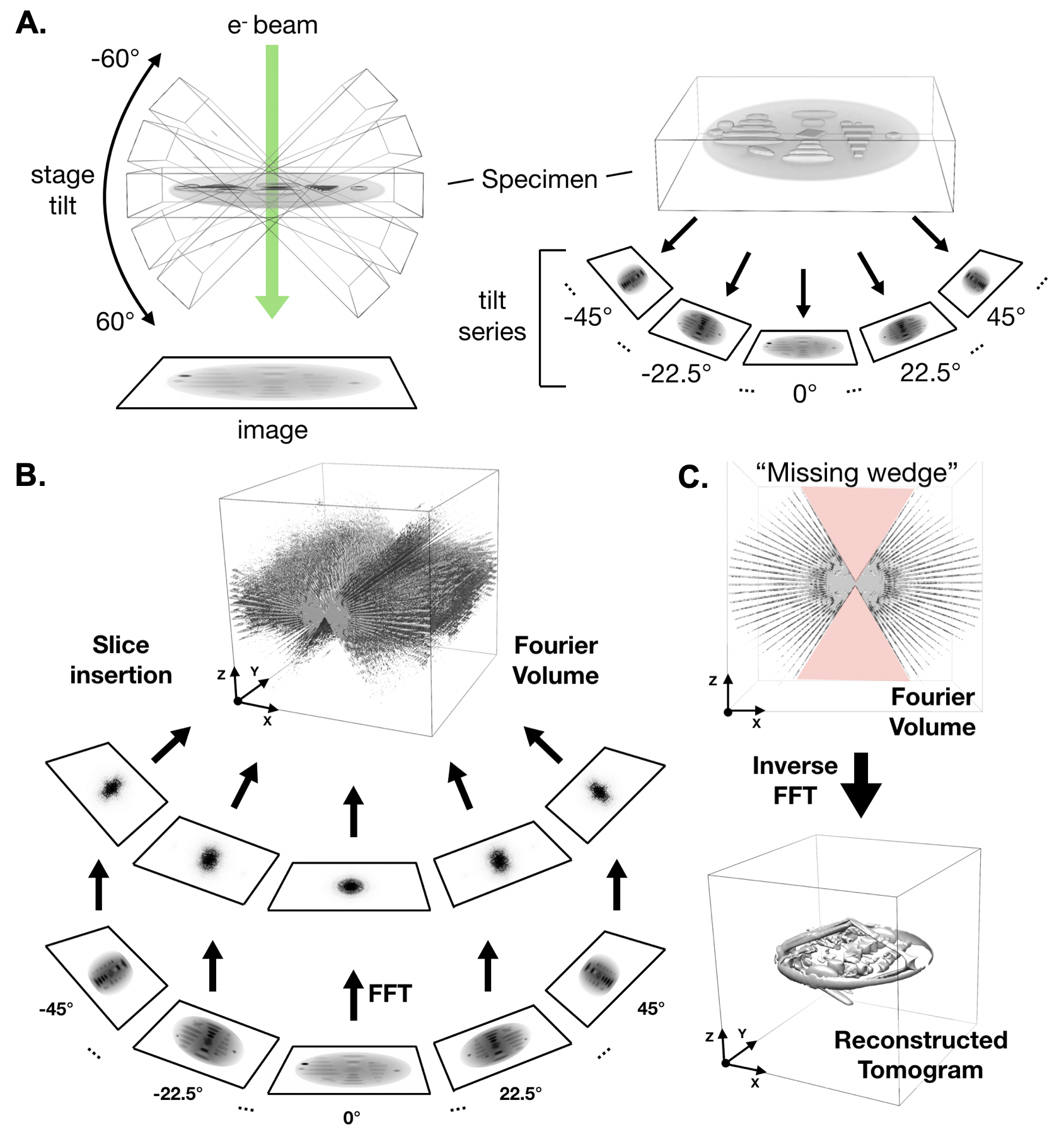
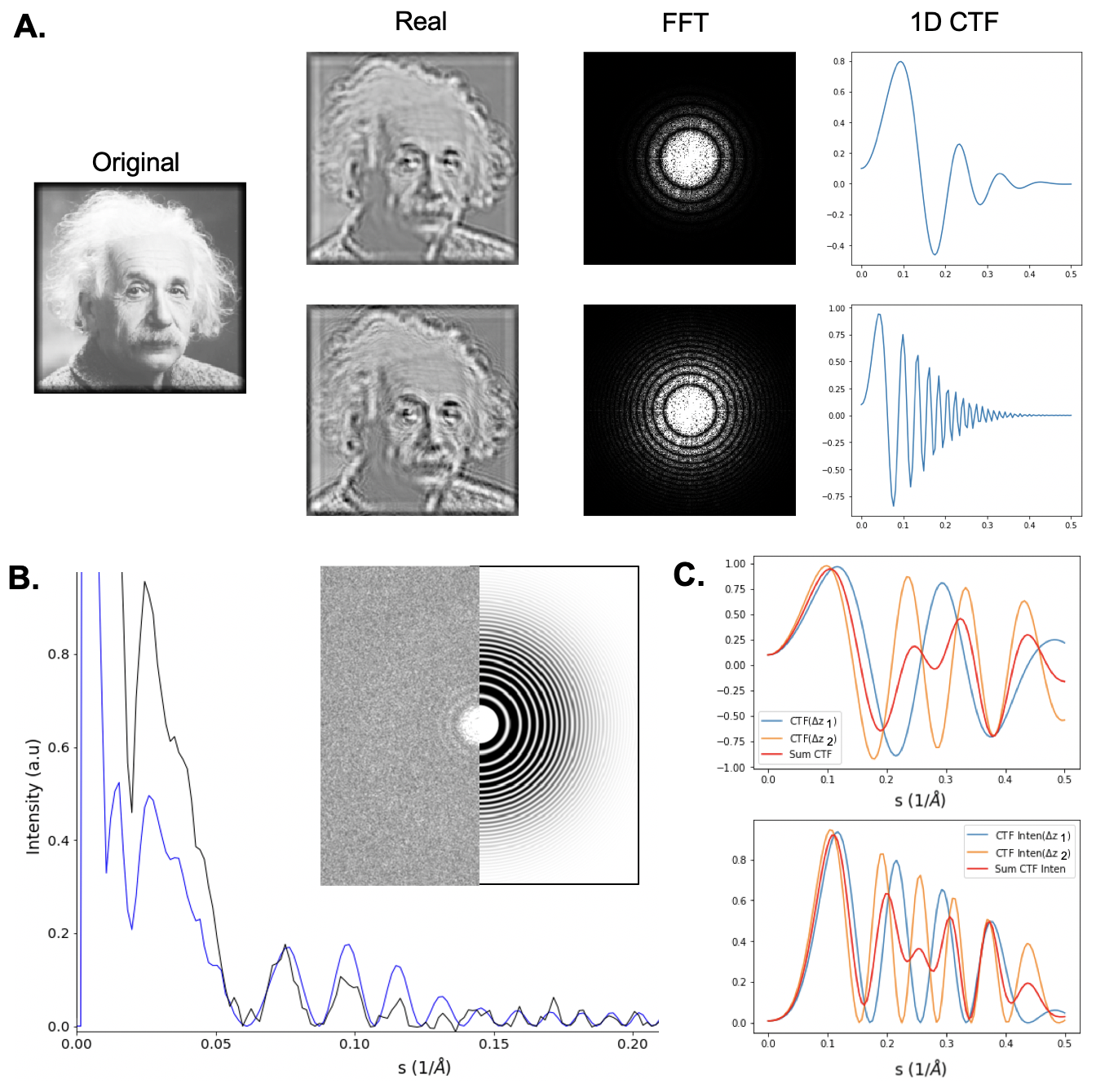
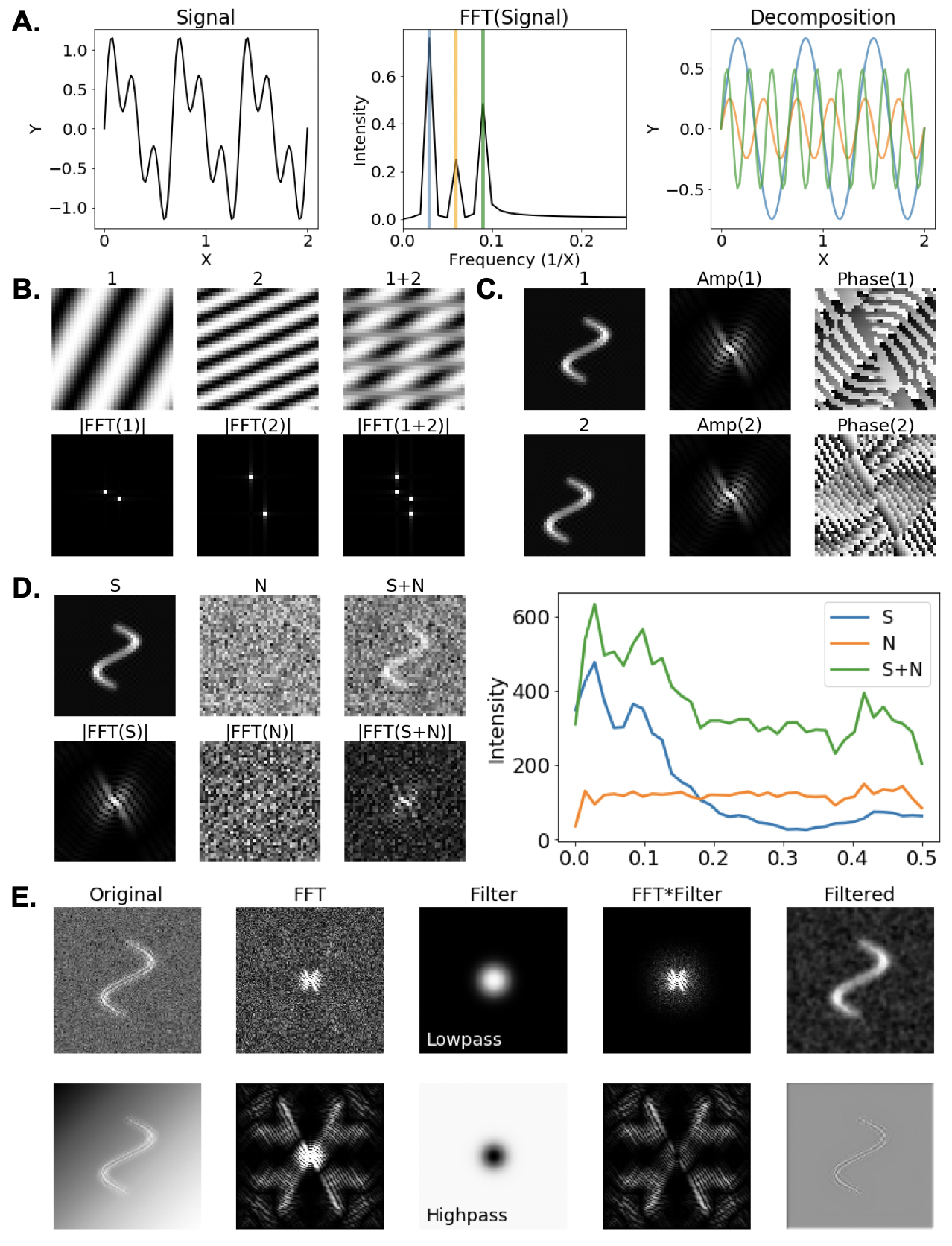
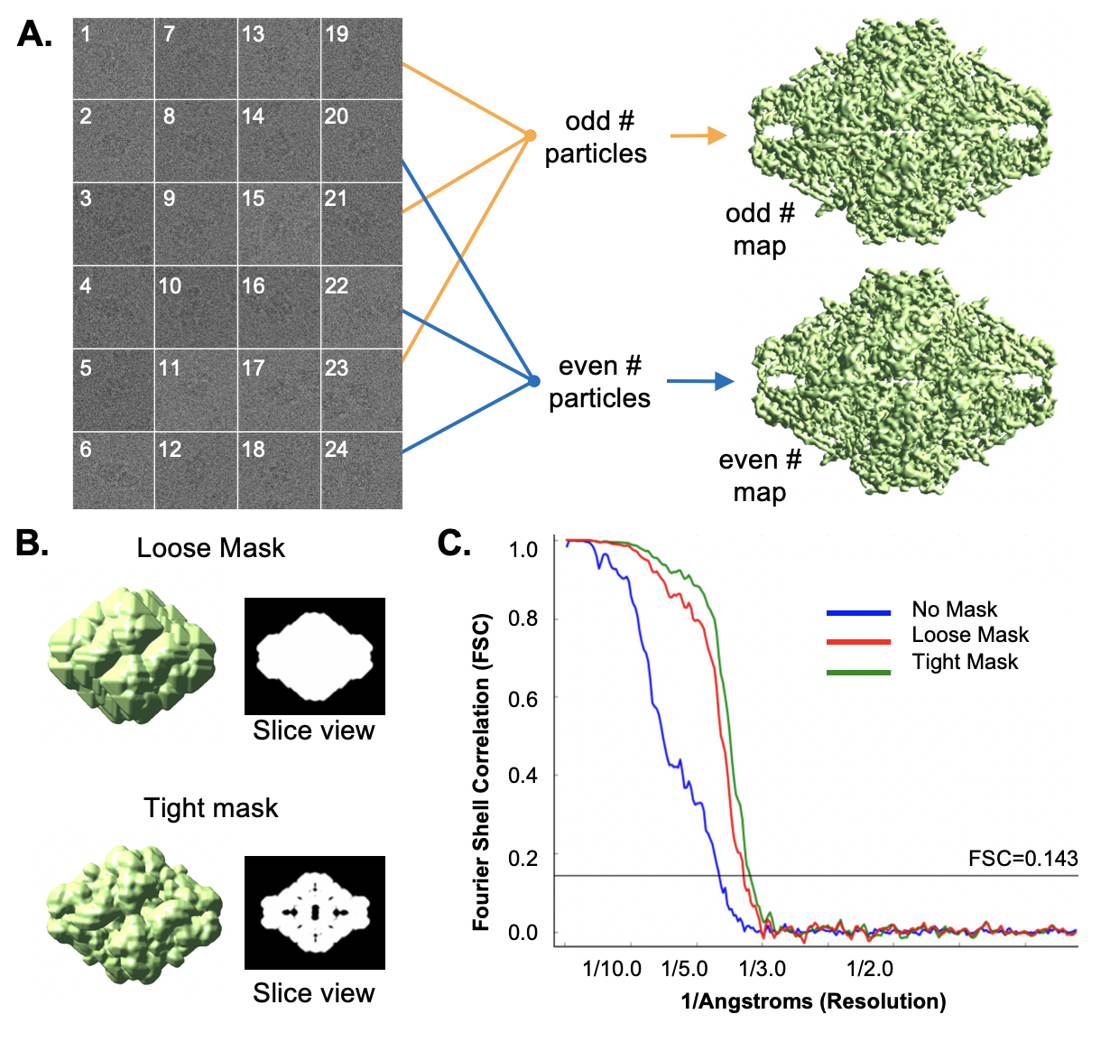
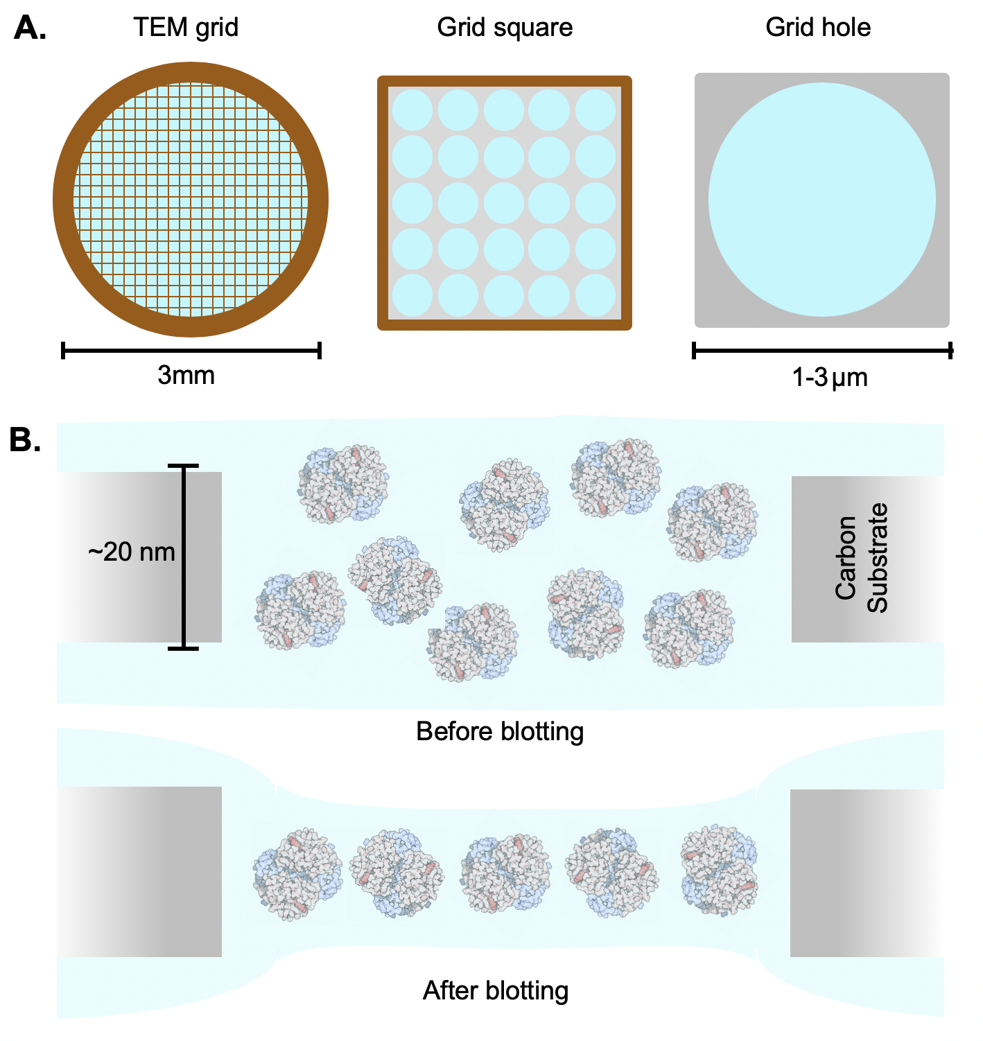
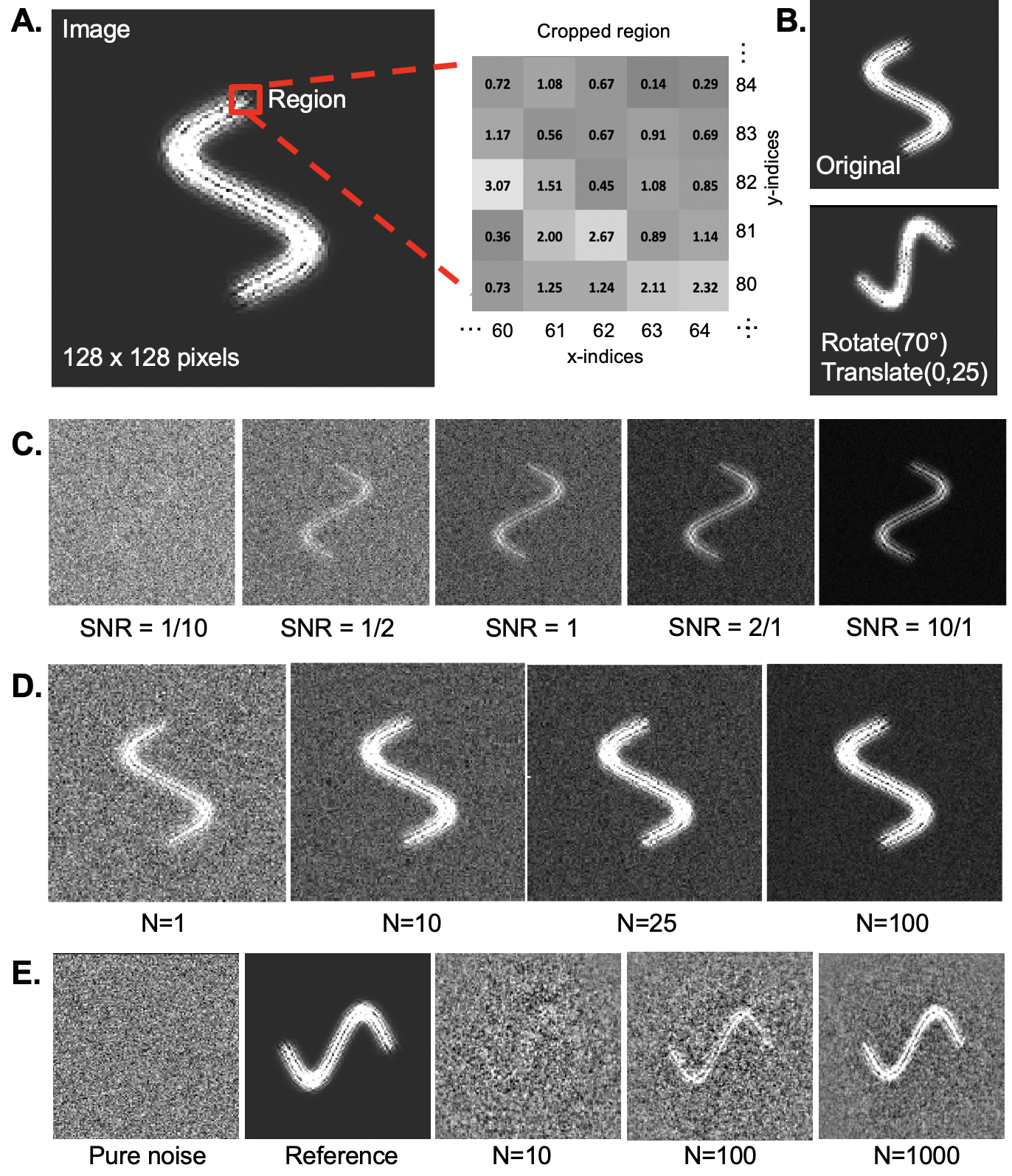
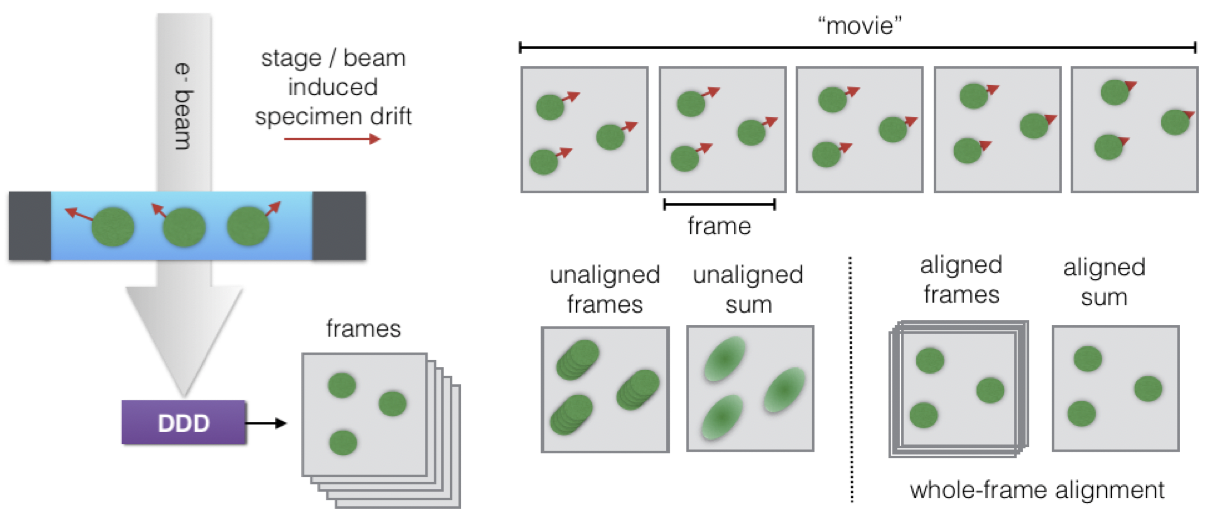
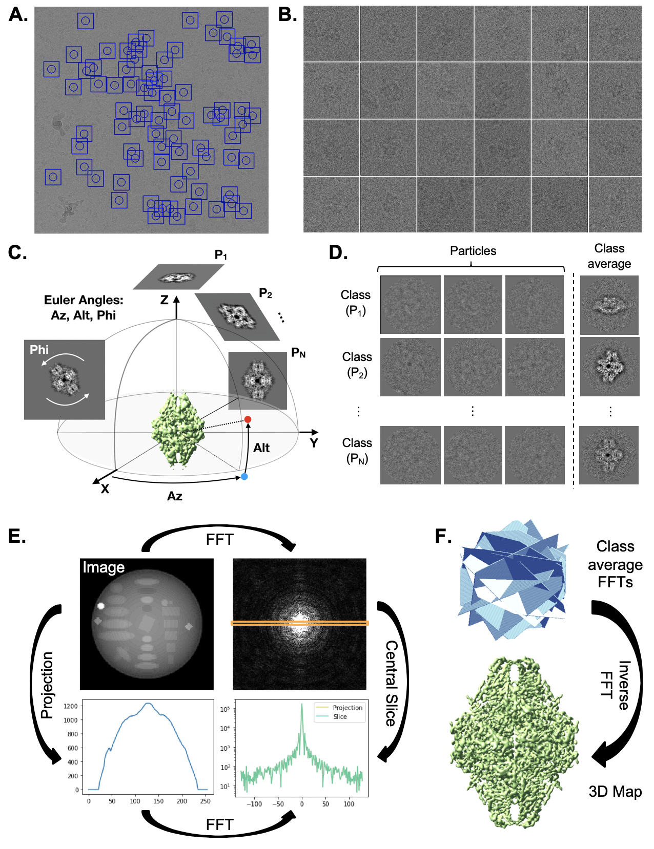
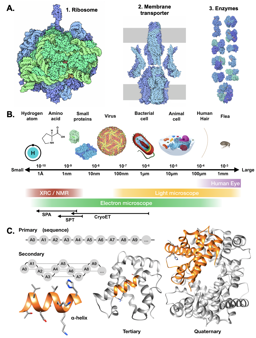
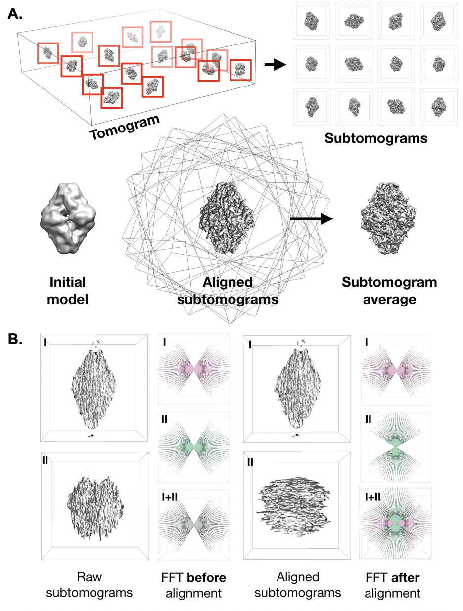
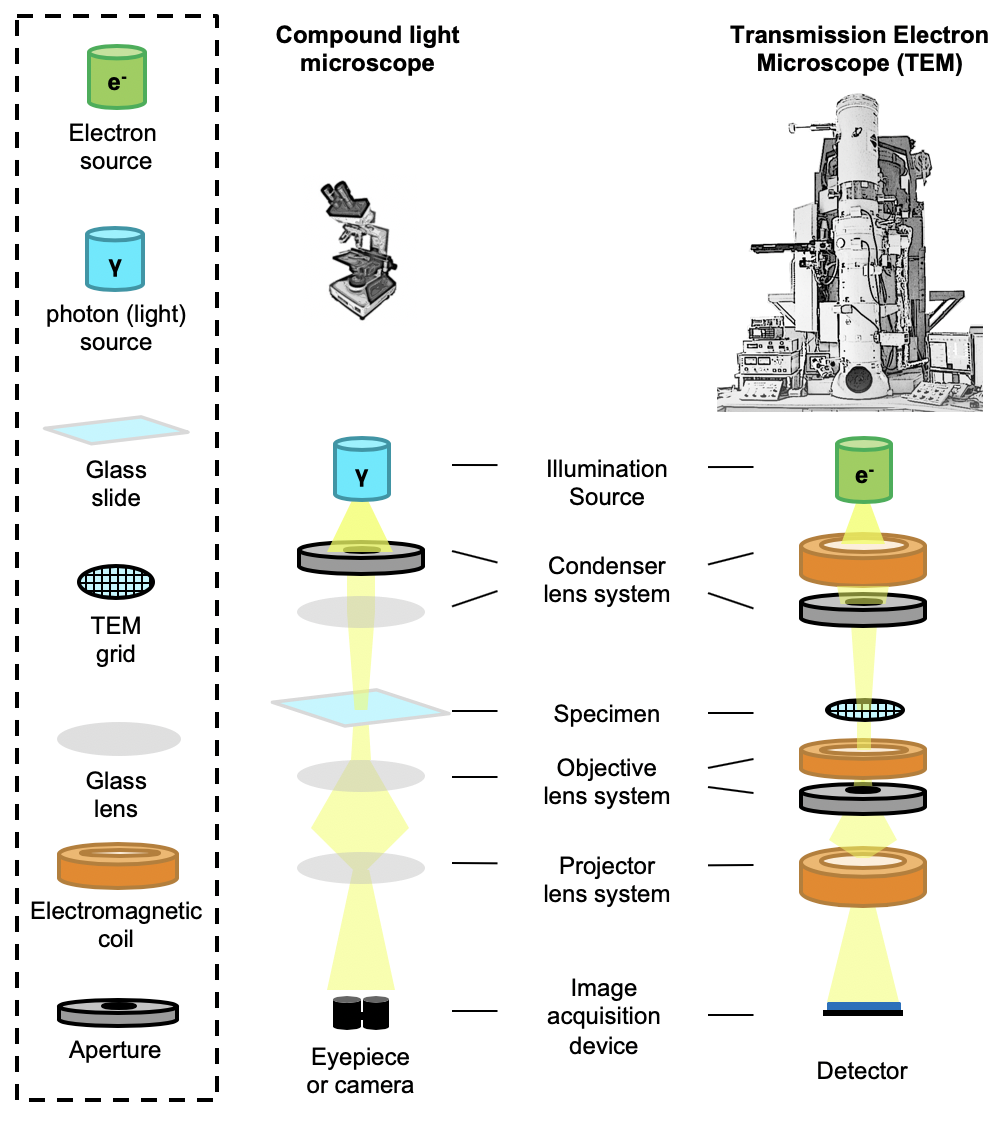
You are not allowed to attach a file to this page.