|
Size: 3006
Comment:
|
← Revision 51 as of 2009-04-11 00:48:59 ⇥
Size: 3933
Comment:
|
| Deletions are marked like this. | Additions are marked like this. |
| Line 2: | Line 2: |
| = 2D = EMAN2 includes a good selection of test images that can be generated in no time at all. They come in many shapes and forms, from simple gradients and shapes to basic noise models. |
= Python test images = EMAN2 includes a good selection of test images. They come in many shapes and forms, from simple gradients and shapes to basic noise models. |
| Line 5: | Line 5: |
| == Using the test_image function in Python == | == test_image (2D) == |
| Line 9: | Line 9: |
| {{{ | {{{#!python |
| Line 23: | Line 23: |
| If you don't specifty the size argument the returned image is 128x128. The following table shows each of the currently defined test_images. | If you don't specify the size argument the returned image is 128x128. The following table shows each of the currently defined test_images. |
| Line 26: | Line 26: |
| ||<:>test_image(0): The EMAN scurve ||<:> test_image(1): Gaussian noise || | ||<:>{{{test_image(0)}}}: The EMAN scurve ||<:> {{{test_image(1)}}}: Gaussian noise || |
| Line 28: | Line 28: |
| ||<:> test_image(2): Dark square ||<:>test_image(3): Light square || | ||<:>{{{test_image(2)}}}: Dark square ||<:>{{{test_image(3)}}}: Light square || |
| Line 30: | Line 30: |
| ||<:>test_image(4): Scurve and random frequency line wave ||<:>test_image(5): Axes || | ||<:>{{{test_image(4)}}}: Scurve and random frequency line wave ||<:>{{{test_image(5)}}}: Axes || |
| Line 32: | Line 32: |
| ||<:>test_image(6): Random frequency line wave ||<:>test_image(7): Scurve and directional gradient || | ||<:>{{{test_image(6)}}}: Random frequency line wave ||<:>{{{test_image(7)}}}: Scurve and directional gradient || |
| Line 34: | Line 34: |
| ||<:>test_image(8): Randomly rotated and translated scurve ||<:>test_image(9): Scurve and Gaussian noise || == Using the processor framework == |
||<:>{{{test_image(8)}}}: Randomly rotated, mirrored and translated scurve ||<:>{{{test_image(9)}}}: Scurve and Gaussian noise || |
| Line 37: | Line 36: |
| == test_image_3d (3D) == At present there are 6 3D test images that are accessible using the test_image_3d function, which is defined in EMAN2.py. {{{#!python #] e2.py Welcome to EMAN2 Prompt provided by IPython Enter '?' for ipython help In [3]: e = test_image_3d(0) In [4]: display(e) }}} The following table shows the currently available 3D test images. ||<:>{{attachment:test_3d_0.png}} ||<:>{{attachment:test_3d_1.png}}|| ||<:>{{{test_image_3d(0)}}}: Axes ||<:>{{{test_image_3d(1)}}}: Spherical waves || ||<:>{{attachment:test_3d_2.png}} ||<:>{{attachment:test_3d_3.png}}|| ||<:>{{{test_image_3d(2)}}}: Tomography test image ||<:>{{{test_image_3d(3)}}}: Solid cube || ||<:>{{attachment:test_3d_4.png}} ||<:>{{attachment:test_3d_5.png}} || ||<:>{{{test_image_3d(4)}}}: Solid sphere ||<:>{{{test_image_3d(5)}}}: Rotated ellipse with holes || = Using the processor framework = == 2D == |
|
| Line 39: | Line 69: |
| {{{ | {{{#!python |
| Line 56: | Line 86: |
| ||{{{ e.process_inplace("testimage.gradient")}}}||{{{ e.process_inplace("testimage.gradient", {'axis','y'}) }}}|| | ||{{{ e.process_inplace("testimage.gradient")}}}||{{{ e.process_inplace("testimage.gradient", {'axis':'y'}) }}}|| |
| Line 64: | Line 94: |
| {{{ | {{{#!python |
| Line 73: | Line 103: |
| {{{ | {{{#!python |
| Line 81: | Line 111: |
= 3D = To come |
Python test images
EMAN2 includes a good selection of test images. They come in many shapes and forms, from simple gradients and shapes to basic noise models.
test_image (2D)
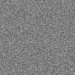
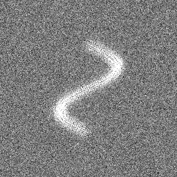
At present there are 10 2D test images that are accessible using the test_image function, which is defined in EMAN2.py.
If you don't specify the size argument the returned image is 128x128. The following table shows each of the currently defined test_images.
|
|
test_image(0): The EMAN scurve |
test_image(1): Gaussian noise |
|
|
test_image(2): Dark square |
test_image(3): Light square |
|
|
test_image(4): Scurve and random frequency line wave |
test_image(5): Axes |
|
|
test_image(6): Random frequency line wave |
test_image(7): Scurve and directional gradient |
|
|
test_image(8): Randomly rotated, mirrored and translated scurve |
test_image(9): Scurve and Gaussian noise |
test_image_3d (3D)
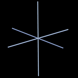
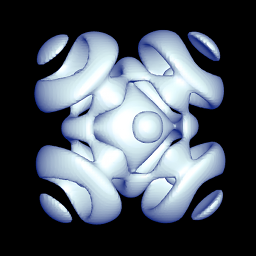
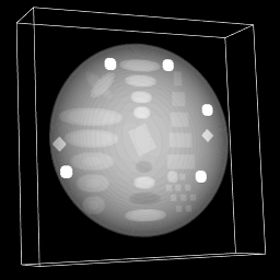
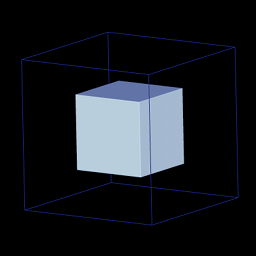
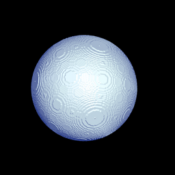
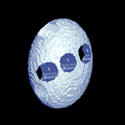
At present there are 6 3D test images that are accessible using the test_image_3d function, which is defined in EMAN2.py.
The following table shows the currently available 3D test images.
|
|
test_image_3d(0): Axes |
test_image_3d(1): Spherical waves |
|
|
test_image_3d(2): Tomography test image |
test_image_3d(3): Solid cube |
|
|
test_image_3d(4): Solid sphere |
test_image_3d(5): Rotated ellipse with holes |
Using the processor framework
2D
To create a test image using the processor framework start by running e2.py and by creating an empty image that is appropriately sized, for example as follows:
Then issue one of the commands shown below in the table to generate the test image
|
|
e.process_inplace("testimage.gradient") |
e.process_inplace("testimage.gradient", {'axis':'y'}) |
|
|
e.process_inplace("testimage.axes") |
e.process_inplace("testimage.circlesphere") |
|
|
e.process_inplace("testimage.scurve") |
e.process_inplace("testimage.noise.gauss") |
Note that this is not all of the test images, and that you can get a complete list by typying e2help.py processors on the command prompt (or see http://blake.bcm.edu/eman2/processors.html). Finally, you can display the image
You can write the image to disk if you need to:
Also, a great many of the test images work on 3D (and 1D) images, so feel free to play around.


