|
Size: 21821
Comment:
|
Size: 21665
Comment:
|
| Deletions are marked like this. | Additions are marked like this. |
| Line 95: | Line 95: |
| == Particle picking == | == Particle picking (10-15 min) == |
| Line 99: | Line 99: |
| * ''Subtomogram averaging -> Manual boxing''' | * '''Subtomogram averaging -> Manual boxing''' Time above is to manually select 30-50 reference particles. |
| Line 101: | Line 101: |
| * ''rename'' the set of boxes to "ribo". This will be used as the label in later stages. * left click and drag to place and reposition boxes in any of the 3 views |
|
| Line 113: | Line 115: |
| == Particle extraction == | == Particle extraction (2 min) == |
| Line 115: | Line 117: |
| In this step, the program will extract unbinned 2D particles from tilt series, perform per particle per tilt CTF correction, then reconstruct individual 3D particles. Select '''Extract particles''' from the left panel, check '''alltomograms''', and specify the label of particle you want to extract. Make sure the label specified here corresponds to the label of particles from the particle boxer. If the box size is correct when you select particles from the GUI, you can leave '''boxsz_unbin''' as -1, so the program will keep that box size. You can adjust the value if you want to change the box size of the extracted particles. If your particles are deeply buried in other densities, using a bigger '''padtwod''' may help, but doing so may significantly increase the memory usage and slow down the process. With CTF information present, it generally does not hurt to check '''wiener''', which filters the 2D particles by SSNR before reconstructing them in 3D. If you want to generate particles without CTF correction, check '''noctf'''. By default, the generated particles will have the same label as they are named in the boxer. If you want to have multiple types of particles, for example, with and without CTF correction, you can specify a different '''newlabel''' each time you launch the program. Specify a binning factor in '''shrink''' to produce downsampled particles if your memory/storage/CPU time is limited, but it may also limit the resolution you achieve at the end. | In this pipeline, the full 1k or 2k tomograms are used only as a reference to identify the location of the objects to be averaged. Now that we have particle locations, the software returns to the original tilt-series, extracts a per-particle tilt-series, and reconstructs each particle in 3-D independently. |
| Line 117: | Line 119: |
| For the EMPIAR example, check '''alltomograms''', and specify the label for the particles (either all ribosome particles or the ones for initial model); click '''Launch'''. | For the tutorial tilt-series: * '''Subtomogram Averaging -> Extract Particles''' * check ''alltomograms'' * enter the label you used when picking particles ("ribo" if you followed the instructions above) * Launch |
| Line 119: | Line 125: |
| Then, go to '''Build set''' in the left panel, check '''allparticles''', and click launch. This will generate particle sets, which are virtual particle stacks that consist of particles with the same label from different tomograms. | * '''Subtomogram Averaging -> Build Sets''' * check ''allparticles'' * Launch * This will generate particle sets, which are virtual particle stacks that consist of particles with the same label from different tomograms. |
| Line 121: | Line 130: |
| For your own data * If the box size is correct when you select particles from the GUI, you can leave '''boxsz_unbin'' as -1, so the program will keep that box size (scaled to the original tilt series) * If your particles are deeply buried in other densities, using a bigger ''padtwod'' may help, but doing so may significantly increase the memory usage and slow down the process. * With CTF information present, it generally does not hurt to check ''wiener'', which filters the 2D particles by SSNR before reconstructing them in 3D. * Specify a binning factor in ''shrink'' to produce downsampled particles if your memory/storage/CPU time is limited, but it will also limit the resolution you can achieve. |
EMAN2 Tomography Workflow Tutorial
- This tutorial is best suited for EMAN2 built after 09/27/2018. Not everything described in the tutorial was functioning yet in the 2.22 release.
This tutorial uses data from EMPIAR: EMPIAR 10064 (only the 4 mixed CTEM tilt series)
- Time estimates for each step are for a well-configured tomography workstation with a high-speed disk, 64+ GB of RAM and 16+ cores.
- The pixel size in the header of the files are incorrect as provided by EMPIAR. The correct Apix value (2.62) should be specified when importing the images.
Prepare input files (~2 minutes)
- Make a new empty folder for the project and 'cd' into that folder
- Make sure any EMAN2 commands you run are executed from within this folder (not any subfolder)
- You may use "Edit Project" from the Project menu to set default values for the project. While not required, it reduces later errors.
- Make sure the workflow mode is set to "TOMO" not "SPR"
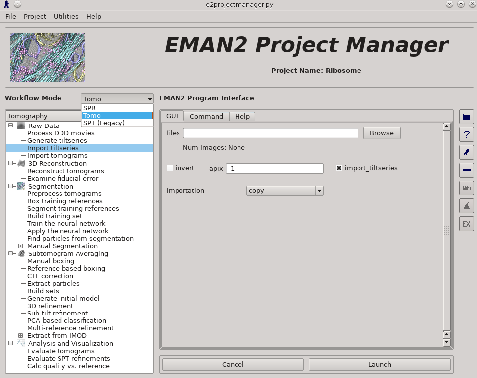
Raw Data -> Import tilt series
Select the files, and make sure importation says copy
In this step you should enter the correct A/pix for your data in the apix box. For EMPIAR10064, this is 2.62. For your own data, you need to know this number. In later steps you should be able to use -1 (default) for apix.
If your tilt series isn't a single stack file, but is many individual images instead, you will need to use Generate tiltseries to build an image stack. This is not necessary for the tutorial data.
Once the options are set, press Launch
It is critical that the filenames for your data not contain any spaces (replace with underscore) or periods (other than the final period used for the file extension). "" (double underscore) is also reserved for describing modified versions of the same file, and should not be used in your original files.
Tiltseries Alignment and Tomogram Reconstruction (20 min)
Alignment of the tilt-series is performed iteratively in conjunction with tomogram reconstruction. Tomograms are not normally reconstructed at full resolution, generally limited to 1k x 1k or 2k x 2k, but the tilt-series are aligned at full resolution. For high resolution subtomogram averaging, the raw tilt-series data is used, based on coordinates from particle picking in the downsampled tomograms. On a typical workstation reconstruction takes about 4-5 minutes per tomogram.
For the tutorial tilt-series:
3D Reconstruction -> Reconstruct Tomograms
check alltiltseries
alternatively you can select one or more tilt series from the tiltseries folder
check correctrot
tltstep = 2
clipz = 64
If you wish to look at the intermediate aligned tilt-series and other files, uncheck notmp
- This is not required for the remaining steps in the tutorial, but can be used to help understand how the tomogram alignment works. This requires significant additional disk space. You may consider doing this for only one tomogram.
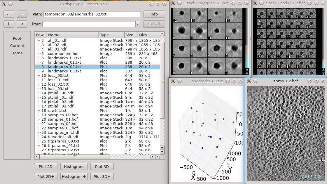
In each tomorecon_XX folder
landmark_0X.txt has the location of the landmarks (which may be fiducials if present) in each iteration
samples_0X.hdf shows the top and side view of those landmarks
ptclali_0X.hdf has the trace of each landmark throughout the tilt series (they should stay at the center of image all the time if the alignment is good)
tomo_0X.hdf is the reconstruction after each iteration
- Launch
When working with your own data:
Either specify the correct tltstep if the tilt series is in order from one extreme to the other, or specify the name of a rawtlt file (as produced by serialem/IMOD).
While the program can automatically compute the orientation of the tilt axis, it is better to fill in the correct value in tltax since there is a handedness ambiguity in the tomogram if determined automatically.
In most cases, the default npk should be fine. If fiducials are present, it is not necessary to adjust this number to match the number of fiducials. The program will use any high contrast areas it finds as potential landmarks.
bytile should normally be selected, as it will normally produce better quality reconstructions at higher speed. If 2k or larger tomograms are created, memory consumption may be high, and you should check the program output for the anticipated RAM usage.
- The graphical interface only permits 1k or 2k reconstruction sizes. In our experience this is normally sufficient for segmentation or particle picking.
When the sample is thin (purified protein, not cells), it is useful to check correctrot to automatically position tomograms flat in ice
It can also be helpful with thin ice to specify a clipz value to generate thinner tomograms (perhaps 64 or 96 for a 1k tomogram).
CTF Estimation (10 min)
For the tutorial tilt-series:
Subtomogram Averaging -> CTF Correction
check alltiltseries
Double check the voltage and cs
- Launch
When working with your own data:
The first two options, dfrange and psrange indicate the defocus and phase shift range to search. They take the format of “start, end, step”, so “2, 5, .1” will search defocus from 2 to 5 um with a step size of 0.1. Units for phase shift is degrees.
For images taken with volta phase plate, we usually have dfrange of “0.2,2,0.1” and psrange of “60,120,2”.
Note that this program is only estimating CTF parameters, taking tilt into account. It is not performing any phase-flipping corrections on whole tomograms. CTF correction is performed later as a per-particle process. This process requires metadata determined during tilt-series alignment, so it cannot be used with tomograms reconstructed using other software packages.
Tomogram annotation (optional)
- Since the tutorial data set is purified ribosomes, this step can be skipped for the tutorial data, and you can move on to template-based particle picking. For cells or other types of complex specimens, tomogram annotation can be used to produce locations of different types of objects.
This section is brief and is only an update to the more detailed tutorial: TomoSeg. Some directory structure and user interfaces have changed in the latest version to match new tomogram workflow as described here:
Segmentation -> Preprocess tomogram
- This step is not always necessary for tomograms reconstructed in EMAN2, but may slightly improve results.
Segmentation -> Box Training References
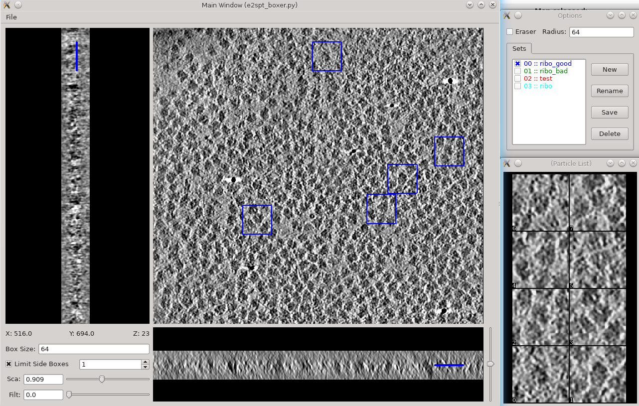
- This is a newer interface than previously used for this step. Select a few "Good" (regions containing the feature of interest) and "Bad" (regions not containing the feature of interest) boxes.
- "~" and "1" on the keyboard can be used to move along the Z axis.
- The new interface permits different types of features to be identified in a single session and in the same tomogram.
If the different features of interest have very different scale, it is always better to keep the box size at 64, and instead rescale the tomogram. As long as the rescaling is done using EMAN2 utilities, the program will correctly keep track of the geometry relative to the original tomogram & tilt series.
- if you are doing this with the tutorial data, you would only have 2 classes of particles "ribo_good" and "ribo_bad".
When pressing Save all visible particles (box checked next to the class name) will be saved
The rest of the annotation process remain unchanged from the original tutorial, except that now, all trained neural networks and training results are saved in the neuralnets folder, and all segmented maps are in the segmentations folder. You now only specify the label of the output file instead of the full file name.
Segmentation -> Find particles from segmentation to turn segmented maps into particle coordinates.
- Input both the tomogram and its corresponding segmentation, and the particles coordinates will be written into the metadata file.
- Slightly tweaking the threshold parameters may yield better results.
featurename will become the label of particles generated. Those particles can be viewed in the particle picking step and processed in the following protocols.
Particle picking (10-15 min)
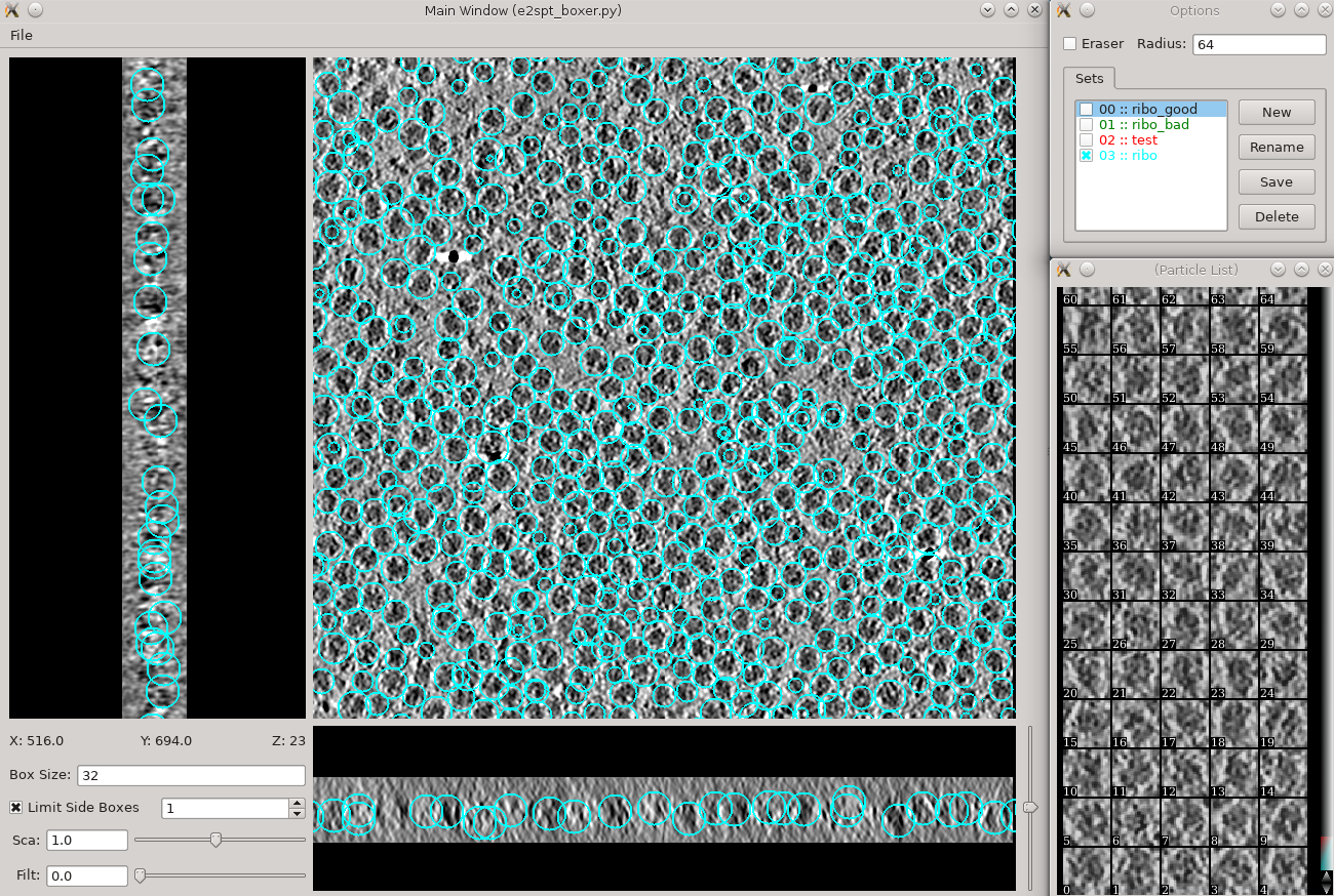
Subtomogram averaging -> Manual boxing Time above is to manually select 30-50 reference particles.
Go through slices along z-axis using ‘~’ and ‘1’ on the keyboard
rename the set of boxes to "ribo". This will be used as the label in later stages.
- left click and drag to place and reposition boxes in any of the 3 views
- Hold down Shift when clicking to delete existing boxes.
- Boxes are shown as circles, which vary in size depending on the Z distance from the center of the particle.
- The interface supports different box types within a single tomogram. Each type has a label. Make sure the label is consistent if selecting the same feature in different tomograms.
- The box size can be set in the main window at the left bottom corner, for the tutorial, use 45 for ribosomes (the unbinned box size is 180).
- If you skipped the tomogram annotation step, we will pick a few particles here to generate an initial model first, and use the initial model as a reference for template matching.
- Select 30-50 particles from a tomogram, then close the boxer window.
- If you have the particle coordinates from tomogram annotation above, you may still wish to do this step to delete any obviously bad particles.
- While you can save 3D particles from the GUI, there is no need to do that here. When you are satisfied with the result, simply close the window.
- You should have ~3000 particles from the 4 tomograms in the dataset.
Particle extraction (2 min)
In this pipeline, the full 1k or 2k tomograms are used only as a reference to identify the location of the objects to be averaged. Now that we have particle locations, the software returns to the original tilt-series, extracts a per-particle tilt-series, and reconstructs each particle in 3-D independently.
For the tutorial tilt-series:
Subtomogram Averaging -> Extract Particles
check alltomograms
- enter the label you used when picking particles ("ribo" if you followed the instructions above)
- Launch
Subtomogram Averaging -> Build Sets
check allparticles
- Launch
- This will generate particle sets, which are virtual particle stacks that consist of particles with the same label from different tomograms.
For your own data
If the box size is correct when you select particles from the GUI, you can leave boxsz_unbin as -1, so the program will keep that box size (scaled to the original tilt series)
If your particles are deeply buried in other densities, using a bigger padtwod may help, but doing so may significantly increase the memory usage and slow down the process.
With CTF information present, it generally does not hurt to check wiener, which filters the 2D particles by SSNR before reconstructing them in 3D.
Specify a binning factor in shrink to produce downsampled particles if your memory/storage/CPU time is limited, but it will also limit the resolution you can achieve.
Initial model generation
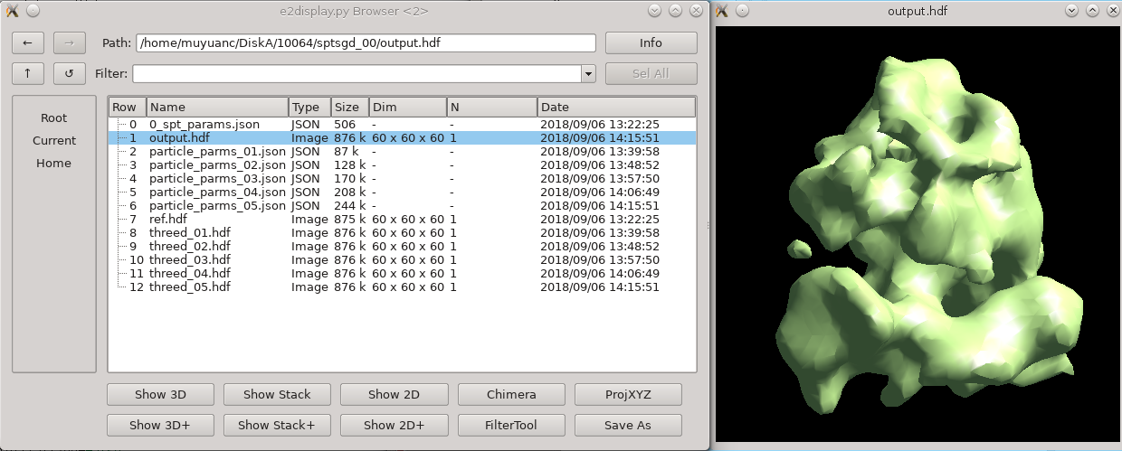
To build an initial model from scratch, simply go to the Generate initial model step and input the particle list. If you wish the process to be faster, set shrink to 2-4. It is not necessary to change other options. The program is parallelized, but not in a standard EMAN2 way. To use more cores, you can enter a bigger number in batchsize. This will not make the program run faster but may make it converge to the correct answer faster. Also using more particles as input won’t make it run faster or slower either, so either input the full particle set if you have them, or the 30-50 particles you pick for the initial model. If the protein is known to be symmetrical, specify the correct symmetry. The program will not actually apply the symmetry (unless you check the applysym box, which is not recommended in general), but it will align the initial model to the symmetry axis so the following steps can work. For most situations, the default number of iterations (niter) of 5 is much more than needed. In this ribosome dataset with
If you generated all particles with tomogram annotation already, skip this step. If not, go to After the program finishes, take a look at the particle coordinates from
Click
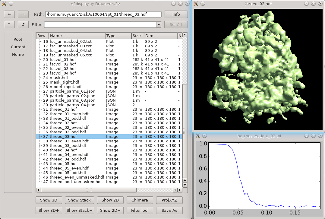
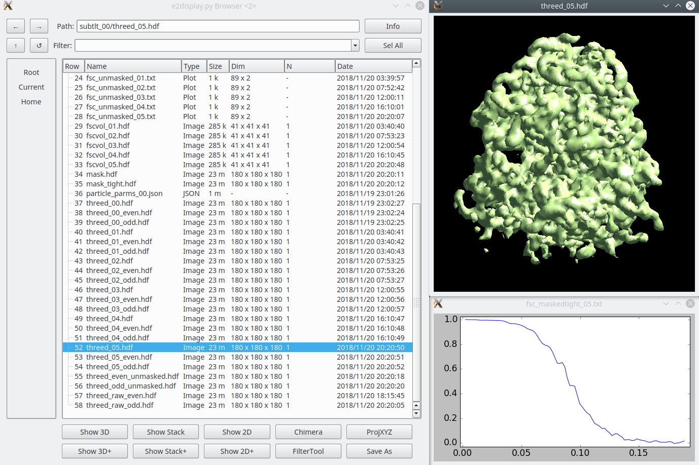
Once the subtomogram refinement finishes, check the final map and FSC curves. In this dataset, you should be able to achieve a resolution of 13-15Å. Now we can refine the orientation of each individual subtilt, i.e. 2D particles from raw tilt series that are reconstructed into to the 3D particles, and push the resolution of the averaged map. Click The default parameters should be generally fine for this dataset, though you may need to alter the
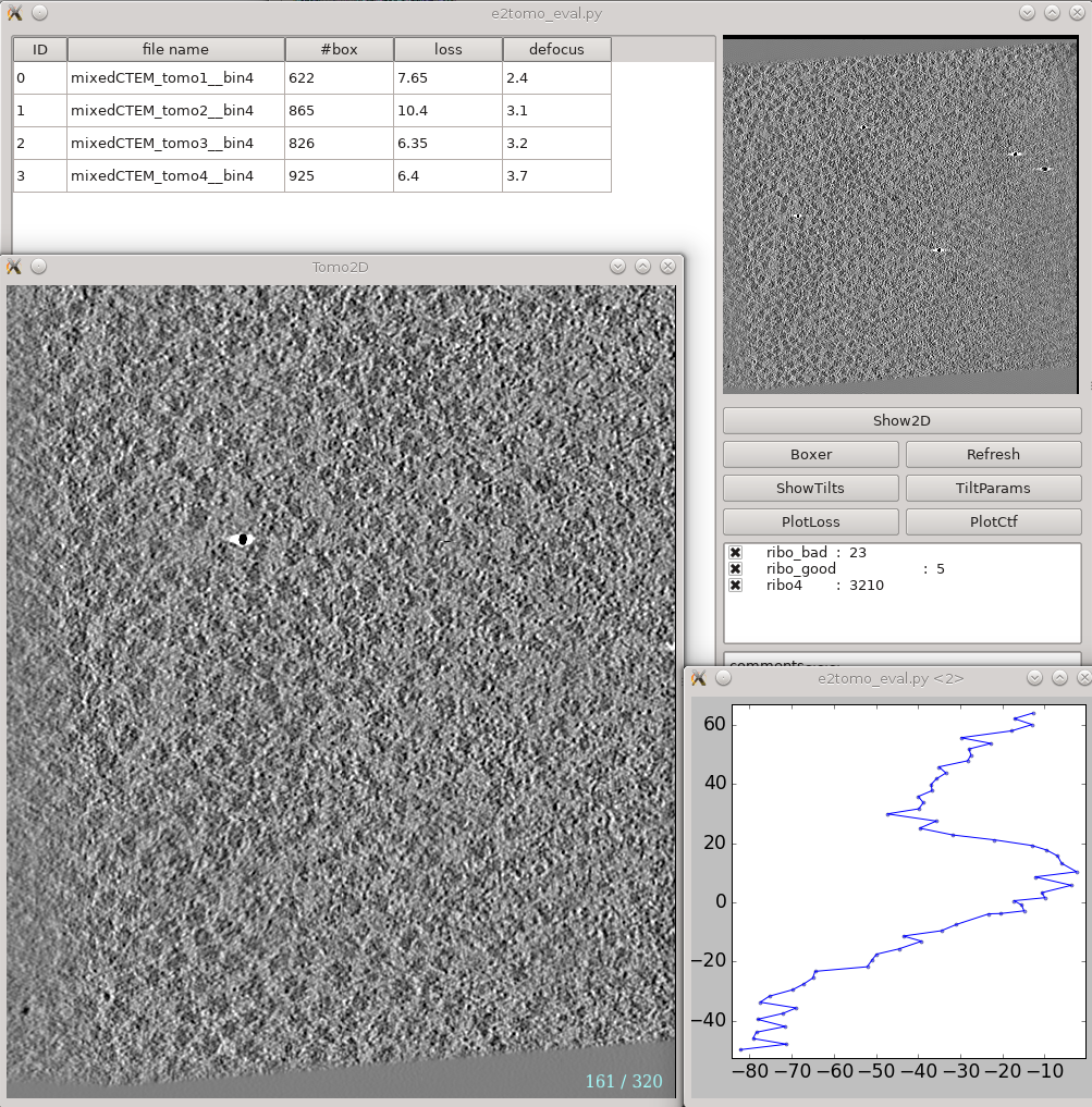
This is a tool that helps you visualize your tomograms with their corresponding metadata, and launch other programs from it. It can be found via On the left is a list of tomograms in the project. Clicking the header of each column will sort the table by that attribute. On the right, the image on the top shows the center slice of the tomogram. The
This tool helps visualize and compare results from multiple subtomogram refinement runs. Launch it from Template matching
Subtomogram refinement
Subtilt refinement
Tomogram evaluation
Refinement evaluation
