|
Size: 13791
Comment: tomobox
|
Size: 13795
Comment:
|
| Deletions are marked like this. | Additions are marked like this. |
| Line 104: | Line 104: |
| * '''ChangeBx''' : Change the box size of positive/negative samples. Ideally, the particles should be recognizable visually from the reference images. The process can be slow if the references come from multiple tomograms. | * '''!ChangeBx''' : Change the box size of positive/negative samples. Ideally, the particles should be recognizable visually from the reference images. The process can be slow if the references come from multiple tomograms. |
| Line 106: | Line 106: |
| * '''TargetSize''' : This controls the size of target area used for CNN training. i.e. particles should be centered in this region in positive samples, and there should not be particle features in this region in negative samples. The region is defined as a Gaussian function and value here is the sigma of the Gaussian. | * '''!TargetSize''' : This controls the size of target area used for CNN training. i.e. particles should be centered in this region in positive samples, and there should not be particle features in this region in negative samples. The region is defined as a Gaussian function and value here is the sigma of the Gaussian. |
| Line 108: | Line 108: |
| * '''PtclThresh''' : The intensity threshold in the neural network output to be recognized as a particle. The target of positive samples should be 1 and negative samples should be 0. * '''CircleSize''' : The radius of circles in pixels on the tomogram slice view. This also controls the closest distance between particles. |
* '''!PtclThresh''' : The intensity threshold in the neural network output to be recognized as a particle. The target of positive samples should be 1 and negative samples should be 0. * '''!CircleSize''' : The radius of circles in pixels on the tomogram slice view. This also controls the closest distance between particles. |
Extra functions for EMAN2 tomography
- This page describes extra functionalities of EMAN2 tomography workflow. This tutorial is frequently updated, so it is better to have EMAN2 version as new as possible.
Focused refinement
Refine local regions of a large complex. Available after 05/23/2019. Still under development.
Start from a successful subtomogram refinement of the full complex (spt_xx folders). For large complexes, it is more convenient to run the full complex refinement with bin2 or smaller particles, then run local refinement with unbinned particles. Here we start from the result from the ribosome tutorial dataset: e2tomo.
Here we follow the Relion single particle multibody refinement paper and focus on the "head" part of the ribosome. From the current subtomogram averaging result, it is quite obvious that the head part has a worse resolution. The great thing about tomography here is that, since we have 3D information of each individual particle, we can just mask out the region we like, instead of doing particle subtraction.
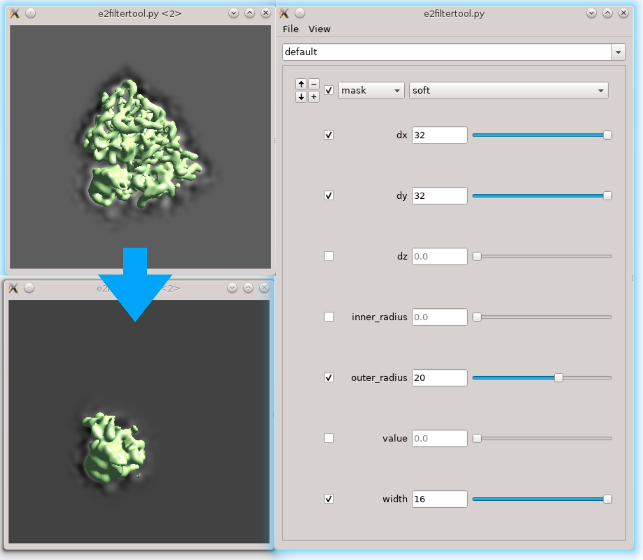
First we need to locate the region of interest. Here we use the filter tool to do it interactively. Run Fitertool on the 3D structure we currently have and insert a mask.soft processor. Play with the parameters. Here I have dx=32:dy=32:dz=0 and the radius of the head part is roughly 36 pixels.

- Now clip the region out and take a look. The box size of the local region needs to be at least 72, but we use 128 regardless because extra padding is always good. Assume we have the result in spt_01 and iteration 5. Run
e2proc3d.py spt_01/threed_05.hdf ref_small_0.hdf --clip 128,128,128,128,128,96
Here the first three numbers after --clip are the box size in x,y,z, and the next three numbers are the center of the box. My original box size is 192, so the center is at 96,96,96. Since we decided that the shift is 32,32,0 in the previous step, the new center should be at 128,128,96.
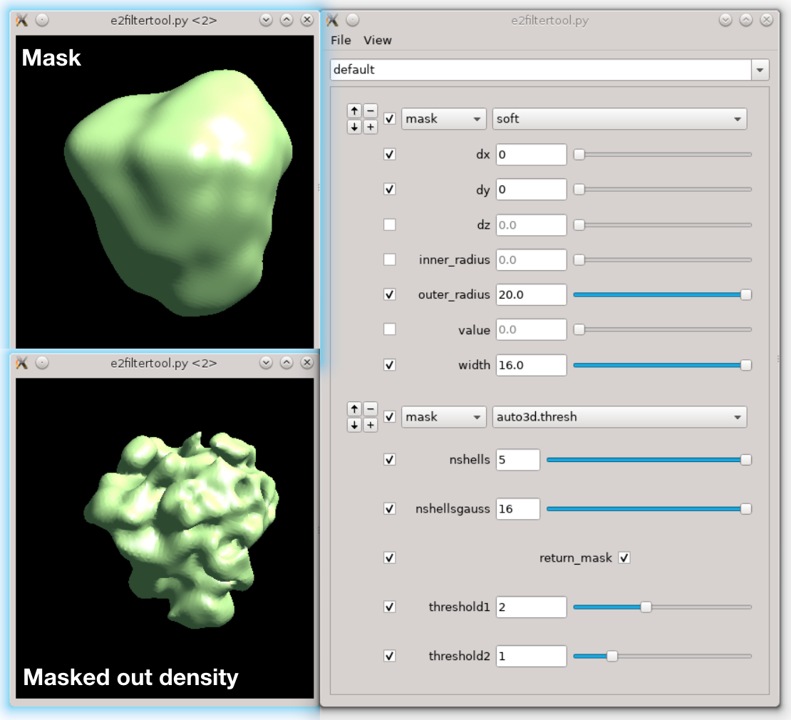
Next we need to make a mask of the region. Open Filtertool on the map we just generated (ref_small_0.hdf), and make a mask you like. Try making the mask as soft as possible but do not touch the edge of the box. Here I use a mask.soft with mask.auto3d.thresh. Once you are satisfied, save the map from Filtertool in File -> Save processed Map. The map will be saved as processed_map.hdf, and we rename it to mask_small_0.hdf. Make sure we save the mask file (with values between 0 and 1), not the masked map. We can also make a masked reference by multiplying the reference with the mask.
e2proc3d.py ref_small_0.hdf ref_small_0_mask.hdf --multfile mask_small_0.hdf

- We also need to prepare the transform input for particle extraction. Open a new text file and write
{'type':'eman', 'tx':32, 'ty':32, 'tz':0}Save the file as xf_small.txt. This seems overcomplicated because this framework also allows local refinement of multiple asymmetrical units individually. For details on how to do this, check the next section.
- Now run particle extraction to get those sub-particles. Run
e2spt_extract.py --jsonali spt_01/particle_parms_05.json --boxsz_unbin 160 --newlabel ribo_small --postxf xf_small.txt --postmask mask_small_0.hdf
Here the program will go back to the original tilt series, extract 2D subtilts and reconstruct the 3D particles. So you can extract unbinned particles even if your initial refinement is done on downsampled particles. The program will deal with scaling automatically. CTF information will also be calculated again, with per-particle defocus at the center of the sub-particles used. The program will not actually align the particles, it will only save the alignment parameters in the header as xform.align3d.
Make a particle set from the newly extracted particles. Here we will have sets/ribo_small.lst. To make sure we are doing everything correctly, average the particles together using the transform in their header.
e2proc3d.py sets/ribo_small.lst avg_ribo_small.hdf --average --averager mean.tomo --avg_byxf
Hopefully, the average should look like the reference we make from the previous subtomogram averaging earlier (you may need to lowpass filter it a bit). If there are many particles, e2proc3d.py can be quite slow as it is single threaded. There is a program in the examples folder that can parallelize the process. If you have examples in your path, run
e2procnd_par.py "e2proc3d.py sets/ribo_small.lst avg_ribo_small.hdf --average --averager mean.tomo --avg_byxf" --threads 24
This also works on most other e2proc2d and e2proc3d processes.
- If everything is working, we can start the refinement run with the particles and the reference.
e2spt_refine.py sets/ribo_small.lst --reference ref_small_0_mask.hdf --niter 5 --maxtilt 45 --refine
You can use any e2spt_refine.py options you like, just make sure to add the --refine option. When the mask used for the particle extraction step is not soft enough, it might affect the missing wedge determination, so setting a --maxtilt seems to be a safer choice.
- This will give us a slightly better alignment on the head part of the ribosome. Once the refinement finishes, we can run a subsequent subtilt refinement based on the subtomogram refinement. There is nothing really different here so just start a run from the GUI. We should get something better than the head part in the original refinement, yet still not quite as good as the large subunit of the ribosome.
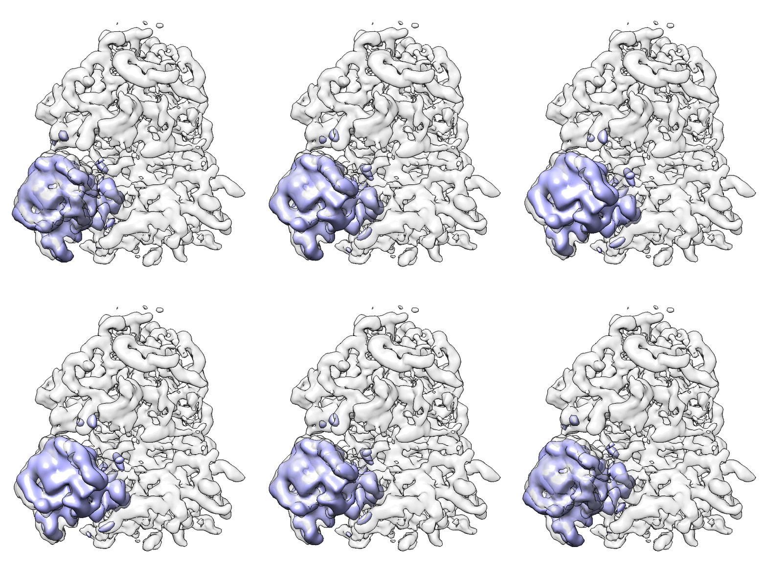
- We can also look at the alignment difference in the focused refinement comparing to the initial full ribosome refinement. An eigen-motion trajectory can be built from the refinement to show how the subunit moves with respect to other parts of the ribosome. Run
e2spt_trajfromrefine.py --path spt_02 --iter 5
We can visualize the motion in Chimera (although I have no idea what is this motion about...).
Focused refinement on multiple asymmetrical units
When you have a complex with multiple asymmetrical units, start from one unit and get the transform and mask following the previous section. Assume we have c5 symmetry and the first unit is at 32,32,0. Then run e2.py and type
sym=Symmetries.get("c5")
xf0=Transform({"type":"eman", "tx":32, "ty":32, "tz":0})
for i in range(sym.get_nsym()):
    xf=sym.get_sym(i)
    print((xf0*xf).get_params("eman"))
You will get a list of transform dictionaries in the printout. Paste them into a text file and use it as the input for particle extraction.
This also works when you have a complex with multiple identical components but does not follow a clear symmetry. Extract each unit individually and align the same reference to the unit. Put the alignment transforms in a text file for particle extraction.
Determine the handedness of a tomogram
In EMAN2 build after 05/23/2019, we can determine the handedness of a tomogram using CTF information. The idea is, at a non-zero tilt angle, one side of the specimen should be closer to the focal plane than the other one. Since this is already taken into consideration in the CTF estimation step, we just run the estimation twice on both the current and inverted hand, and check which one has a better fit.
Find a tilt series in the dataset with good signal (at least 2 clear Thon rings). This will only work when the defocus can be determined unambiguously in the first place, so phase plate data may and may not work... Reconstruct it with tltax set empty so the program will determine the tilt angle automatically.
Run the CTF estimation from the GUI using the correct parameters, but check the checkhand option. The program will suggest whether the hand need to be inverted at the end.
If the hand is flipped, reconstruct the tomograms with the suggested tltax value given by the CTF estimation program.
Automated particle selection
In EMAN2 build after 02/01/2020, a new tool is implemented for CNN guided automated particle selectin from tomograms. The concept is similar to the tomogram segmentation protocol, but a number of changes have been made to improve the accuracy and throughput of the process. A new GUI has been made to simplify the training process. Note that this requires a CUDA compatible GPU and tensorflow setup to work. To use, run
e2spt_boxer_convnet.py --label xxx
Here label will be the label of the newly selected particle. This will bring up three windows: the main window with various options and a list of tomograms, and two windows (should be empty in the beginning) for positive and negative samples. Clicking any tomogram in the list will bring up two other windows: the slice view of the tomogram and the list of particles under the given label.
To start, select a few (>5) positive to negative samples. On the tomogram slice view, left-click to select positive samples, and Ctrl+left-click to select negative samples. Shift-click an image in the sample list to delete it. The particles should be well-centered in the positive samples, and there should not be particles in the center of negative samples. Click Train to start training and some output will be printed in the command line. Keep clicking Train (or use a larger Niter) until the loss stops decreasing (or whenever you want to stop). Then click Apply to let the program select particles using the trained network. Go through the particle list, Ctrl+left-click a falsely recognized particle to add it to the list of negative samples (left-click a particle will add it to the positive samples, but it is not very necessary since they are selected by the network already). You can also go through the tomogram again to add a few particles that are not selected by the network into the positive samples. Click Train again to re-train the network using the new training set, and click Apply to inspect its results. Repeat the process until the neural network's performance is satisfying. You can also select other tomograms in the list, to test the performance of the model and add more positive/negative samples to the training set. Finally, go through all tomograms in the list and apply the network to select the particles. These particles can be viewed and modified in e2spt_boxer.py, and extracted through the particle extraction steps of the main workflow.
Description of items on the GUI:
New/Save/Load: Initialize a new CNN / save the current trained network to disk / load a trained network from disk.
ChangeBx : Change the box size of positive/negative samples. Ideally, the particles should be recognizable visually from the reference images. The process can be slow if the references come from multiple tomograms.
Reference/Particle selection box: Display circles of references or particles in the tomogram slice view.
TargetSize : This controls the size of target area used for CNN training. i.e. particles should be centered in this region in positive samples, and there should not be particle features in this region in negative samples. The region is defined as a Gaussian function and value here is the sigma of the Gaussian.
Learnrate : Learning rate for the CNN training. Normally no need to change this...
PtclThresh : The intensity threshold in the neural network output to be recognized as a particle. The target of positive samples should be 1 and negative samples should be 0.
CircleSize : The radius of circles in pixels on the tomogram slice view. This also controls the closest distance between particles.
Sum/Max selection box : Choose between different modes of the loss function. Sum is used for globular particles that are generally confined in the target area. In Max mode, the CNN only assume there are particle features that exist within the region. It is harder to train than the Sum mode, but allows particles of irregular shapes, such as protein fibers.
Map particles to tomograms
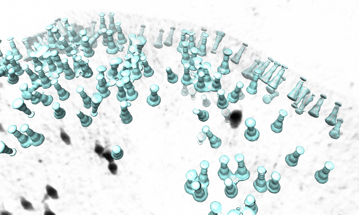
There is a simple tool to map the averaged structure to the determined position and orientation of each particle in a tomogram. Available after EMAN2.3. In versions after 05/23/2019, the function is moved to the Analysis and Visualization section in the GUI.
Subtomogram Averaging -> Map particles to tomograms
Set path to be one of the spt_XX folder (not the subtlt ones).
Set iter to be the iteration you want to use from the refinement.
- Browse for one tomogram you want to map the particles to.
The program will then find all particles in the selected tomogram that are used in the refinement, map the averaged structure back, and produce a file called ptcls_in_tomo_xx_yy.hdf, where xx is the name of tomogram and yy is the number of iteration used. This is sometimes quite useful for objects in cellular environment (when membrane proteins are obviously upside down for example). Image rendered with Chimera.


