|
Size: 6598
Comment:
|
Size: 6541
Comment:
|
| Deletions are marked like this. | Additions are marked like this. |
| Line 1: | Line 1: |
| This is for the new subtomogram-subtilt refinement pipeline that will become available after EMAN2.9. Currently on the [[https://github.com/cryoem/eman2/tree/spt_new |spt_new]] branch in Github. Both the pipeline and the tutorial are still under construction. Backward compatibility of the results is not guaranteed... | This is for the new subtomogram-subtilt refinement pipeline that is available in Github and continuous build after EMAN2.91 (03/09/2021). Both the pipeline and the tutorial are still under construction. Backward compatibility of the results is not guaranteed... |
This is for the new subtomogram-subtilt refinement pipeline that is available in Github and continuous build after EMAN2.91 (03/09/2021). Both the pipeline and the tutorial are still under construction. Backward compatibility of the results is not guaranteed...
Tomogram reconstruction
- New patch tracking mode to support FIB data with few landmarks. Specify --patchtrack=1 or 2 to run on 512 or 1k tilt series images. This also works as a pre-alignment step before the standard iterative alignment, and can improve the result in some cases where there are large drifts during the tilt series.
- The patch tracking mode also includes automatic tomogram positioning. This should in theory work better than the --correctrot option, as it positions based on the sample instead of the fiducial plane.
- Initial coarse alignment and the first iteration of iterative alignment are also reworked. The behavior should be more stable when large drifts are present.
Particle selection
Subtomogram-subtilt refinement
- The subtomogram and subtilt refinement routines have been reworked and now become an integrated and iterative process. 3D particle orientation, 2D subtilt translation/rotation, defocus variation can be refined in the same loop.
Optimizers from Scipy are used instead of home-made aligners. They seem to have slightly better convergence.
Correlated local particle motion is also considered which greatly boosts the resolution of the averaged structure. It is worth noting that the concept similar to the M paper, but with different implementations.
To use, simply run
e2spt_refine_new.py --ptcls sets/ptcls.lst --ref reference.hdf --iters p,p,t,r,p,d
Most of the options of the program follow the same convention as e2spt_refine.py. For example, use --goldstandard to specify starting resolution for gold standard refinement, use --setsf for structure factor-based amplitude correction, add --tophat to use one of the local filter options.
Control the iterative refinement with the --iters option, where different characters denote different types of refinement. p for 3D particle orienation, t for 2D subtilt translation, r for subtilt translation & rotation, and d for subtilt defocus refinement.
- Adjust the weight of local particle motion using --smooth and --smoothN. For each individual particle, --smoothN controls how many of its neighbors are considered to model the local motion, and --smooth controls how much the neighboring particles are weighted during the alignment. The weight of neighboring particles decays in a Gaussian form based on the distance to the center particle of consideration. --smooth=0 means only the center particle is considered, and the program should perform in a similar way as the original subtilt refinement. The default --smoothN is 15 and --smooth=100, which seem to work well in the tutorial dataset.
- --ssnrwt weights the subtilt particles based on their SSNR to the reference during the 3D reconstruction. It is only applied at the last iteration since it may introduce some mask bias to the results.
For each round, there will be an aliptcls2d_xx.lst file that records the transform of each subtilt. Only iterations marked as p produces aliptcls3d_xx.lst file, which will be used for the later iterations of subtilt refinement.
- The actual fraction of particle kept should be around (--keep)^3. That is, when --keep=.9, it removes the worst 10% 3D particles, 10% 2D subtilt with the worst score, and 10% of subtilt with the largest drift.

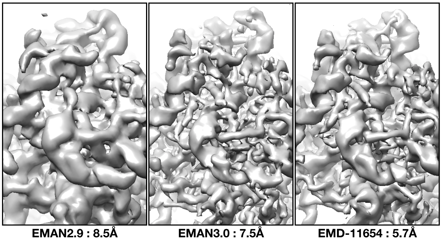
With default options, the tutorial dataset should be able to get to ~7.5Å resolution. While the reported number is lower, the features in the resulting map are about as good as EMPIAR-11654.
Visualize particle motion in individual tilts
After a refinement, run
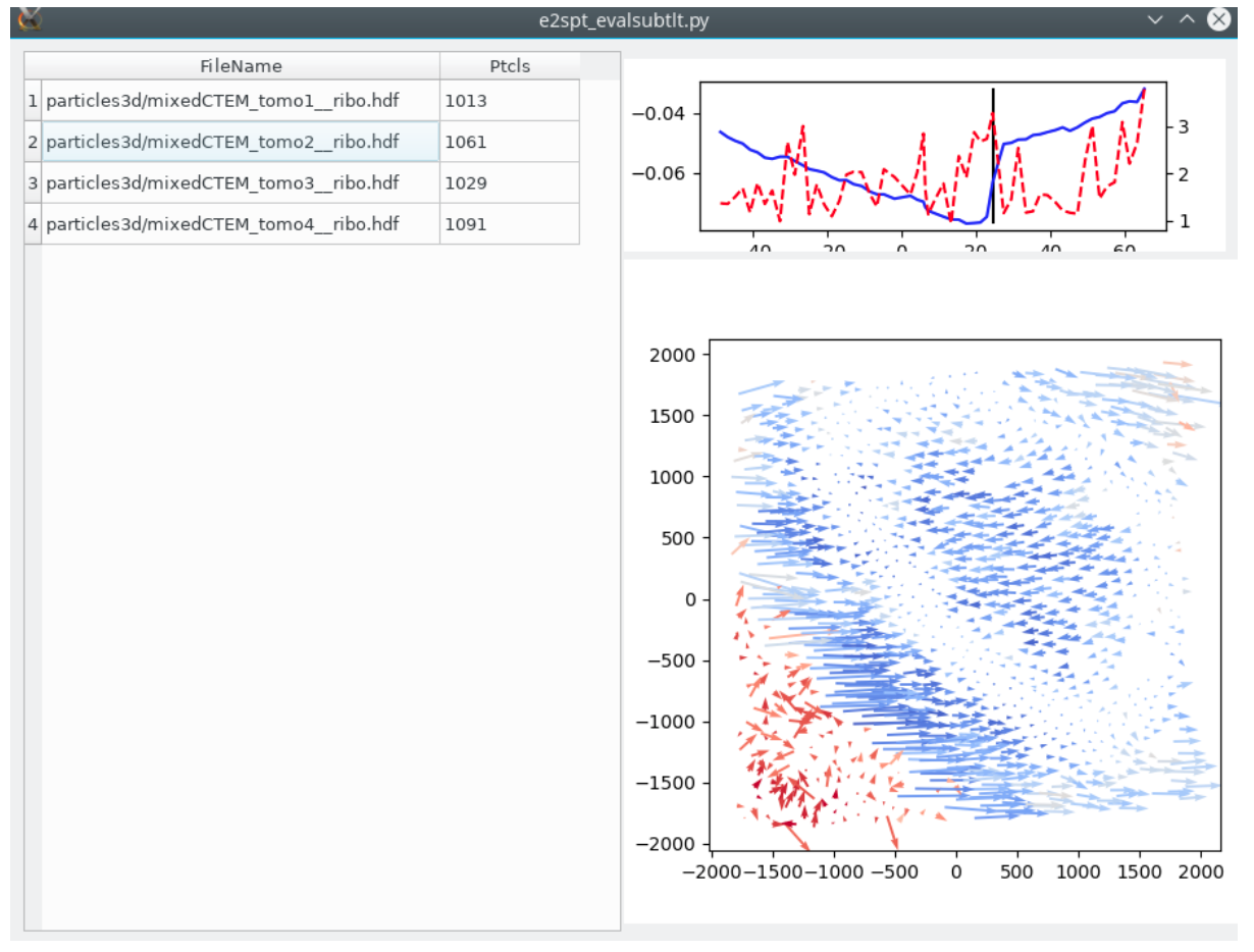
e2spt_evalsubtlt.py --path spt_xx --loadali2d <last aliptcls2d_xx.lst file> --loadali3d <last aliptcls3d_xx.lst file>
It will take a while to load all metadata, and plot the trajectory of each particle on each tilt image in each tomogram.
In the top panel, the blue curve represents the average score of all 2D particles in that tilt, and the red curve represents the average distance of the subtilt motion with respect to the alignment of the 3D particle. The quiver plot below shows the trajectory of each individual particle, colored by its alignment score.
Focused refinement and continuous motion
After a refinement run, make a customized mask for the domain of interest using the filter tool, then generated the masked referenced. Make sure to mask both the even and odd maps that will be used as references and name them properly.
e2proc3d.py spt_xx/threed_yy_even.hdf spt_xx/threed_yy_masked_even.hdf --multfile mask_smallunit.hdf
e2proc3d.py spt_xx/threed_yy_odd.hdf spt_xx/threed_yy_masked_odd.hdf --multfile mask_smallunit.hdf
Do another short run with the masked reference with the --localrefine option. Load the last aliptcls2d and aliptcls3d file from the last run use the corresponding options. In this case, using --iters=p,t will be enough.
e2spt_refine_new.py --ptcls sets/ptcls.lst --ref spt_xx/threed_yy_masked.hdf --iters p,t --startres 7 --goldcontinue --loadali2d spt_xx/aliptcls2d_yy.lst --loadali3d spt_xx/aliptcls2d_yy.lst --mask mask_smallunit.hdf --localrefine
Then, run
e2spt_trajfromrefine --path spt_xx --ali3dold spt_xx/aliptcls3d_00.lst --ali3dnew spt_xx/aliptcls3d_01.lst --ali2d spt_xx/aliptcls2d_00.lst
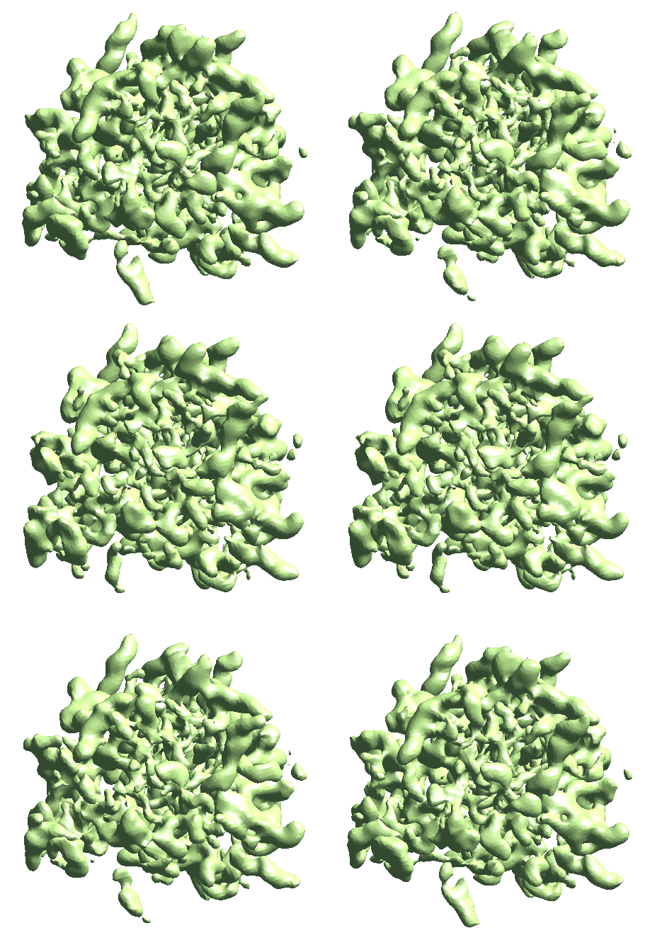
Note that since we want to look at the motion of the masked domain within the coordinates of the original refinement, here use the old aliptcls2d.lst file. If the goal is to visualize the motion of other parts of the protein with the focused part fixed, use the newer aliptcls2d file. The program will output two 3D map stacks corresponding to the trajectories of the first two eigenvectors. They can be filtered/masked manually with e2proc3d.py before visualization.


