Tomogram Annotation/Segmentation
Availability: EMAN2.2+, or daily build after 2016-10 This is the tutorial for a Convolutional neural network(CNN) based semi-automated cellular tomogram annotation protocol.
If you are using this in a publication, please cite:
M. Chen et al. (2017). Convolutional Neural Networks for Automated Annotation of Cellular Cryo-Electron Tomograms. Nature Methods, http://dx.doi.org/10.1038/nmeth.4405
A stable (thus not up-to-date) online version of the tutorial can also be found at Protocol exchange: https://www.nature.com/protocolexchange/protocols/6171
Updates:
10/2018: Now it uses Tensorflow backend which should be included during installation. Also particle boxing interface and directory structure are updated to incorporate into the new e2tomo pipeline.
01/2018: Slides of a recent tutorial in Rutgers boot camp can be found here. tomoseg_tutorial_rutgers.pdf
- 10/2017: We have switched to gpuarray backend for CUDA9 support. It should still work with CUDA7.5+ and the old cuda backend in Theano.
Installation
CNN based tomogram annotation makes use of the TensorFlow deep learning toolkit. At the time of this writing, tensorflow effectively requires CUDA, the compute framework on NVidia GPUs. While future support for OpenCL (an open alternative to CUDA) seems likely, and while it is possible to use TensorFlow on a CPU, at present we cannot recommend running this tool on Mac/Windows. You may do so, but training the networks may be VERY slow.
To make use of accelerated TensorFlow, your machine must be properly configured for CUDA. This is outside the installation of EMAN2, and requires specific drivers, etc. on your machine. Some extra information on how to use CUDA and GPU can be found at http://blake.bcm.edu/emanwiki/EMAN2/Install/BinaryInstallAnaconda#Using_the_GPU
Setup workspace
If you used EMAN2 for your tomogram alignment/reconstruction (EMAN2/e2TomoSmall), simply 'cd' to the project folder and launch e2projectmanager.py. If you will be using tomograms produced by other software:
Make an empty folder and cd into that folder at the command-line. Run e2projectmanager.py.
Select the Tomo Workflow Mode.
Import or Preprocess
If your tomograms were produced using the EMAN2 workflow:
- You should preprocess your tomograms to prepare them for segmentation.
Select Segmentation -> Preprocess Tomograms
Press Browse, Sel All then OK
All of the other options should normally be fine, and you can press Launch
If your tomograms were produced by other software, and you wish to do the segmentation in EMAN2:
- If your original tomograms are in multiple folders, you can repeat the next step.
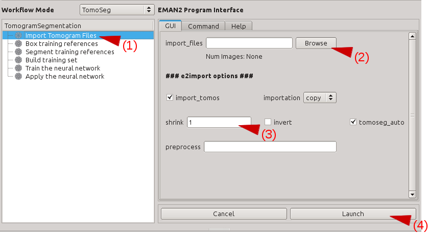
Select Raw Data -> Import Tomograms
Use Browse to select all of the tomograms you wish to segment, and press OK
EMAN2 uses the convention that tomograms have "dark" or negative contrast, and individual particles and 3-D averages will have "white" or positive contrast. If your tomograms have positive contrast (features look bright when displayed) check the Invert box.
If your tomograms are larger than ~1k x 1k, you should consider downsampling, or Shrinking them for segmentation. Normally 1k x 1k is more than sufficient for accurate segmentation. ie - if your original tomograms are 4k x 4k, enter 4 in the shrink box.
- In deciding how much to shrink the original tomograms, it is only important that the features you wish to recognize are still recognizable by eye. If shrinking produces a tomogram where a feature you wish to identify is only 1-2 pixels in size, then you are shinking too much.
Launch
- Once imported, you should preprocess your tomograms to prepare them for segmentation.
Select Segmentation -> Preprocess Tomograms
Press Browse, Sel All then OK
All of the other options should normally be fine, and you can press Launch
- Note: There may be cases where it is impossible to pick a single scale which works well to annotate features at different scales. For example, if you are trying to annotate icosahedral viruses (large scale) and actin filaments (require small scale to identify) in the same tomogram, you may need to import the tomogram twice, with 2 different "shrink" factors, segment each feature at the appropriate scale, then rescale/merge the final segmentation maps. This is a topic for advanced users, and we encourage you to learn the basic pipeline with a single feature before attempting this.
Overview
The network training process may seem complicated at first, but in reality it is extremely simple. You will be training a neural network to look at your tomogram slice by slice, and for each pixel it will decide whether it does or does not look like part of the feature you are trying to identify. This feature is termed the Feature of Interest (FOI). To accomplish this task, we must provide a few manual annotations to teach the network what it should be looking for. We must also provide some regions from the tomogram which do not contain the FOI as negative examples. That is, you are giving the network several examples of: "I am looking for THIS", and several more examples of: "It does NOT look like THIS".
For the network to perform this task well, it is critical that you be absolutely certain about the regions you select for training. The largest error people make when training the network is to include regions containing ambiguous density. If you select a tile containing a clear feature you wish to include, but the tile also contains some density you are unsure of, then you will be in a difficult situation. If you mark the ambiguous region as a particle, and it actually is something else, the trained network will not be very selective for the FOI. If you do not mark the ambiguous density, and it turns out to actually be the FOI, then you are trying to train the network to distinguish between the object you said was the ROI and the object you said was not (but was), which may cause a training failure, or a network which misses many FOIs. The correct solution is not to include any tiles containing ambiguous density! Only include training tiles you are certain that you can annotate accurately in 2-D.
There will be other cases where it may be difficult to distinguish between two features. For example, at low resolution, the strong line of an actin filament, may look somewhat like the edge of a membrane on an organelle. If you train only a single network, and it is trained to recognize actin, then you apply it to a cellular tomogram, you will likely find many other features, such as membrane edges, and possibly the edge of the holy carbon film, get mis-identified as actin. While you may be able to more carefully train the actin network, or alter the threshold when segmenting, usually the better solution is to train a second network to recognize membranes and a third network to recognize the C-film hole, then compete the 3 networks against one another. While the vesicle may look somewhat like actin at low resolution, it should look more like a vesicle than actin, so the result of the competitive networks will be a more accurate segmentation of all 3 features.
We will begin the tutorial by training only a single network. You can then go back and follow the same process to train additional networks for other features, then finally at the end, use a program designed to compete these solutions against one another.
Select Training Examples
In this stage we will be manually selecting a few 64x64 pixel tiles from several tomograms, some of which containing the feature of interest (FOI) you wish to train the neural network to identify. We will identify some 2-D tiles which contain the FOI and other tiles which do not contain the FOI at all. In the next step we will annotate the tiles containing
Select Box training references. Press browse, and select the preproc version of any one imported tomogram. Leave boxsize as -1, and press Launch. In a moment, three windows will appear: the tomogram view, the selected particles view, and a control-panel (labeled Options). Unlike the 2-D particle picking interface used in single particle analysis, which is almost identical, this program allows you to move through the various Z-slices of the tomogram. The examples you select will be 2-D, drawn from arbitrary slices throughout the 3-D tomogram. Additionally, this program permits selecting multiple classes of tiles from the same tomogram. For example, you may have one class of tiles containing the FOI and another class which does not contain the FOI. It is critical that you use a consistent naming convention for these different classes of particles, since we would like to have training references from multiple tomograms used for the network training. In the window named e2spt-boxer, make sure your box size is set to 64. The Options window also contains the number 64, but this is the radius for the eraser, and its value does not matter. In the options window you should see a list with something like particles_00 in it. The tile selecting program can be used to select several different "classes" of particles from the same image/volume. Select this first element in the list and press Rename. Call this first set good_1. If you go back and select tiles for a second FOI, you would call those tiles good_2. Note that there is nothing magical about this name, but it needs to be self consistent among different tomograms. Press the New button, and rename the new set bad_1. We will use this to select tiles which do not contain the FOI at all Click on good_1 to make it the selected set, then: In the window containing your tomogram, begin selecting boxes. You can move through the slices of the tomogram using the vertical slider in the lower right corner of the tomogram window, and zoom in and out with the scroll wheel. Select and reposition tiles with the left mouse button. Hold down shift when clicking to delete existing tiles. As you select tiles, they will appear in the (Particles) window. Highlight bad_1 When you are done selecting good and bad references from a single tomogram, go back to the Options window, and put a checkmark next to only the good_1 set. Then press Save. Accept the provided default name. Repeat this process for bad_1: put a check next to only bad_1 and press save. You have now created two new files in the particles/ folder. You may repeat this process for other tomograms spanning the defocus range in your project. Each time you do this you will create a pair of new files in particles/ Note: The box size for training tiles MUST be 64x64. If the feature of interest does not fit in a 64x64 tile, you will need to create a more down-sampled copy of your tomogram for the recognition to work well. You can do this manually with e2proc3d.py. If you create a down-sampled version of a tomogram, use the exact same name and location as the original tomogram, but add a suffix to the name preceded by 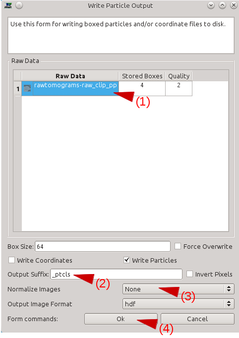
Manually Annotate Samples
The next step is to manually identify the FOI
Segmentation -> Segment training references
particles should be set to the good_1 file you just created in the particles/ folder.
output -> leave blank
segment -> leave this checked
Launch
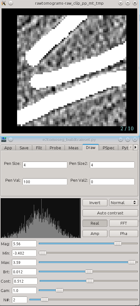
Two windows will appear, one containing images, and the other a control panel. You can navigate through the images using the up/down arrows, or using the N# slider . The control panel will open with the Draw tab selected.
- Using the left mouse button, draw on each of the FOI to exactly cover the feature of interest as best you can. If necessary you can always can go back to the FOI selection window to check the surroundings of each feature to insure accurate segmentation
- Generally speaking, the CNN can recognize the FOI if you can recognize the same feature in 2D patches by eye without ambiguity.
The key in this step is consistentcy. If you annotate a feature in a particular way you should annotate other features in the same way. If the pen is too large, reduce both Pen Size and Pen Size2.
- Ideally you should be pixel-accurate in this process, but a small amount of 'slop' at the edges is likely inevitable, and should not pose a major problem. It IS critical however, that you correctly annotate all possible FOIs in every frame. If you miss a single FOI, it may significantly degrade the performance of the network. That is, if your annotation is consistently a little larger than the FOI, this will pose much less of a problem than completely missing a single FOI in the training tiles.
- When you are finished, simply close the windows. The segmentation file will be saved automatically as "*_seg.hdf" with the same base file name as your ROIs.
Build Training Set
This step is simply combining the files we have created through this step in a specific way to prepare for network training.
Segmentation -> Build training set
particles_raw -> select particles/*_good_1.hdf
particles_label -> select particles/*_good_1_seg.hdf
boxes_negative -> select particles/*_bad.hdf
trainset_output -> leave blank
ncopy -> default of 10 should be fine. This controls the number of randomly oriented training replicas to create
Launch
This will create a new file with _trainset appended to the name. It takes only a few seconds to run.
Train Neural Network
Segmentation -> Train the neural network
trainset -> the particles/*_trainset file you created in the previous step
device -> If you are running on a machine with CUDA properly configured with Tensorflow, enter GPU in this box. Otherwise you will have to use CPU
defaults should be fine for all other options, Launch
If you use cpu this process may take a long time to run. On a GPU it should take 15-20 minutes.
- Any errors or other issues will appear in the console window where you ran e2projectmanager.
- If you get an error, for example:
terminate called after throwing an instance of Xbyak::Error
zsh: killed e2tomoseg_convnet.py
This generally means you have an incompatible version of TensorFlow installed in your environment. It may be incompatible with the version of CUDA or the driver installed on your computer, or there may be some other fundamental incompatibility. If you encounter this, you can try:
conda install tensorflow-gpu or conda install tensorflow-cpu as appropriate to update to the latest version.
If you need to go to an intermediate version, such as 1.9 (which seems to have pretty good forwards and backwards compatibility at the time this is being written, you can append =1.9 to either of the previous commands
if you continue to encounter problems, the commands: nvidia-smi and nvcc --version can give you more information. You may then want to report the issue to the EMAN2 mailing list for help.
- If you get an error, for example:
- If the program runs correctly, you will see "Training..." on the console. The first time you train a network there may be a several minute delay, but eventually numbers will begin to appear in the console. If these numbers are extremely large, it implies something is wrong. Contact us for help if you have issues.
- After the training is finished, it is recommended to look at the training result before proceeding.
Open the trainout_*.hdf using the EMAN2 file browser. You should see something like:
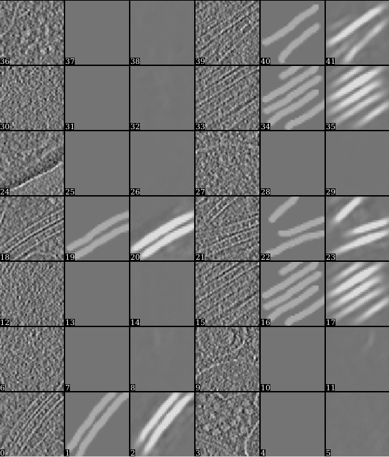
- Zoom in or out a bit so there are 3*N images displayed in each row. For each image triplet, the first one is the tile from the tomogram, the second is the corresponding manual segmentation, and the third is the neural network output for the same FOI after training. The neural network is considered well trained if the third image matches the second image reasonably well. For the negative particles, both the second and the third images should be largely blank (the 3rd may contain some very weak features, this is ok).
- If the training result looks completely wrong, go back and check your positive and negative training set first. Most significant errors are caused by training set errors, i.e. having some positive particles in the negative training set, or one of the positive training set is not correctly segmented.
If the training result looks suboptimal (the segmentation is not clear enough but not totally wrong), you may consider continuing the training for a few rounds. To do this, go back to the Train the neural network panel, choose the previously trained network for the from_trained box and launch the training again. It is usually better to set a smaller learning rate in the continued training. Consider change value in the learnrate to ~0.001, or the displayed learning rate value at the last iteration of the previous training.
Once you are satisfied with the result, go to the next step to segment the whole tomogram.
Apply to Tomograms
Finally, open Apply the neural network panel. Choose the tomogram you used to generate the boxes in the tomograms box, choose the saved neural network file (not the "trainout_" file, which is only used for visualization), and set the output filename. You can change the number of threads to use by adjusting the thread option. Keep in mind that using more threads will consume more memory as the tomogram slices are read in at the same time. For example, processing a 1k x 1k x 512 downsampled tomogram on 10 cores would use ~5 GB of RAM. Processing an unscaled 4k x 4k x 1k tomogram would increase RAM usage to ~24 GB. When this process finishes, you can open the output file in your favourite visualization software to view the segmentation.
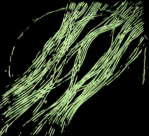
To segment a different feature, just repeat the entire process for the each feature of interest. Make sure to use different file names (eg - _good2 and _bad2)! The trained network should generally work well on other tomograms using a similar specimen with similar microscope settings (clearly the A/pix value must be the same).
Merging multiple annotation results
Merging the results from multiple networks on a single tomogram can help resolve ambiguities, or correct regions which were apparently misassigned. For example, in the microtubule annotation shown above, the carbon edge is falsely recognized as a microtubule. An extra neural network can be trained to specifically recognize the carbon edge and its result can be competed against the microtubule annotation. A multi-level mask is produced after merging multiple annotation result in which the integer values in a voxel identify the type of feature the voxel contains. To merge multiple annotation results, simply run in the terminal:
mergetomoseg.py <annotation #1> <annotation #2> <...> --output <output mask file>
Tips in selecting training samples
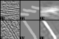
- Annotate samples correctly, as a bad segmentation in the training set can damage the overall performance. In the microtubule case, if you annotate the spacing between microtubules, instead of the microtubules themselves (it is actually quite easy to make such mistake when annotating microtubule bundles), the neural network can behave unpredictably and sometimes just refuse to segment anything. Here is the training result on an incorrect and correct segmentation in one training set. Note the top one (22) is annotating the space between microtubules.
- Make sure there are no positive samples in the negative training set. If your target feature is everywhere and it is hard to find negative regions, you can add additional positive samples which include various features other than the target feature (annotating only the target feature).
- You can bin your tomogram differently to segment different features. Just import multiple copies of raw tomogram with different shrink factors, and unbin the segmentation using math.fft.resample processor. It is particularly useful when you have features with different lengthscales in one tomogram, and it is impossible to both fit the large features into a 64*64 box and still have the smaller features visible at the same scale.
- In some cases, there is a significant missing wedge in the x-y plane slices (you can visualize this by clicking Amp button when looking at the slices in EMAN2). So the resolvability on x direction is different than that on y direction. It is important to provide features running in different directions in the training set, otherwise the neural net may only pick up features in one direction based on the Fourier patten. Also, you may want to check the stage of the microscope, since this may suggest the sample is not tilted exactly around the x axis.
- It is also vital to cover various states of the target feature. For example, if you want to segment single layer membranes, you may want to have some cell membrane, some small vesicles, and some vesicles with darker density inside, so the neural network can grab the concept of membrane. Just imagine how you would teach someone with no biological knowledge about the features you are looking for. On the other hand, it is possible to ask the neural network to separate different types of those same features. In the membrane example, it is possible to train the neural network to segment vesicles from cell membranes based on the curvature, or recognize dense vesicles based on the difference of intensity on both side of the membrane, given carefully picked training set.
Acknowledgement
Darius Jonasch, the first user of the tomogram segmentation protocol, provided many useful advices to make the workflow user-friendly. He also wrote a tutorial of the earlier version of the protocol, on which this tutorial is based.
