|
Size: 33216
Comment:
|
Size: 33183
Comment:
|
| Deletions are marked like this. | Additions are marked like this. |
| Line 163: | Line 163: |
| There is a newer tool which can be used for deep-learning based particle picking, which is really a different task than annotation. If you have a GPU and prefer this over the reference based approach outlined in the next section, see: [[[https://blake.bcm.edu/emanwiki/EMAN2/e2tomo_more#Automated_particle_selection|New automatic particle picking]]. The annotation tool is still functional and available, but is targeted more at annotation of cellular features: [[http://eman2.org/Programs/tomoseg| TomoSeg]] | There is a newer tool which can be used for deep-learning based particle picking, which is really a different task than annotation. If you have a GPU and prefer this over the reference based approach outlined in the next section, see: [[EMAN2/e2tomo_more#Automated_particle_selection|New automatic particle picking]]. The annotation tool is still functional and available, but is targeted more at annotation of cellular features: [[http://eman2.org/Programs/tomoseg|TomoSeg]] |
EMAN2 Tomography mini-Workflow Tutorial
This version of the EMAN2 Tomography Pipeline tutorial is designed to run on well equipped laptops or standard workstations, unlike the full tutorial which requires a well-equipped tomography workstation. It should be possible to complete this tutorial in a reasonable time on a computer with 16 GB of ram and 4 cores, but resolution will be limited to ~15 A, not the subnanometer resolution provided by the main tutorial.
- This tutorial is best suited for EMAN2 built after 09/27/2018. Not everything described in the tutorial was functioning yet in the 2.22 release.
- This version of the tutorial is based on a subset of reduced sampling data from the same EMPIAR data set as the main tutorial. This should be downloaded from the EMAN2 website. The pixel size for this data is 3.93 A/pix.
- To cite:
- Chen, M., Bell, J.M., Shi, X. et al. A complete data processing workflow for cryo-ET and subtomogram averaging. Nat Methods 16, 1161–1168 (2019)
Documentation of some newly developed tools can be found in TomoMore.
There is now a newer pipeline for integrated subtomogram and subtilt refinement. Some documentation can be found in TomoNew (frequently updated).
Computer Requirements
- This reduced version of the tutorial can be completed on a well equipped laptop or standard desktop workstation.
- Minimum recommended configuration (timing estimates based on single quad-core computer):
- 16 GB RAM
4 cores @ >2 ghz
- 40 gb free disk space
- a high performance disk (SSD or RAID) will significantly reduce runtimes
Note: Anyplace in EMAN2 where you are requested to enter the number of threads to use, you should specify the number of cores your machine has. Computers are often advertised as 4 core/8 thread or 8 core/16 thread. Trying to run image processing using this advertised number of threads will usually make processing run slower, not faster. You may optionally increase the number of cores by ~25%, ie - on a 4 core machine, 5 may be a reasonable number to specify.
Download Data
Download the data from the EMAN2 Tutorials page
Prepare input files (~2 minutes)
- Make a new empty folder for the project and 'cd' into that folder
- Make sure any EMAN2 commands you run are executed from within this folder (not any subfolder)
- You may use "Edit Project" from the Project menu to set default values for the project.
If you downloaded our prepared data set, it will already contain an info folder containing the project settings, so you should not need to change anything.
- For this project use 3000 kDa, 2.7 mm Cs, 300 keV and 3.93 A/pix.
- The mass need not be precise, it is only used to keep isosurface values roughly self-consistent.
- Make sure the workflow mode is set to "TOMO" not "SPR"
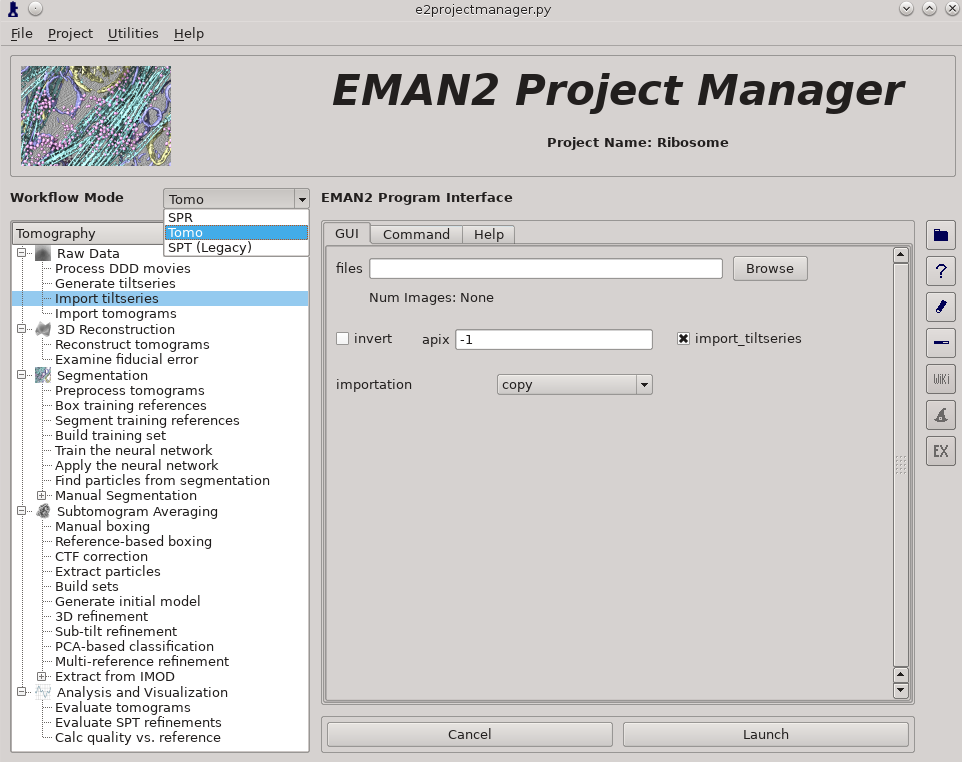
Raw Data -> Import tilt series
Files -> select the 3 provided .hdf files
rawtlt, mdoc -> leave these blank
invert should not be selected
apix = 3.93, in later steps you can use -1, which tells it to use the known value
import_tiltseries = selected
importation = copy
compressbits = 5 (8 is fine as well, but will make file sizes slightly larger)
Once the options are set, press Launch
When working with your own data:
- It is critical that the filenames for your data not contain any spaces (replace with underscore) or periods (other than the final period used for the file extension).
"__" (double underscore) is also reserved for describing modified versions of the same file, and should not be used in your image filenames.
If your tilt series isn't a single stack file, but is many individual images instead, you will need to use Generate tiltseries to build an image stack
Tiltseries Alignment and Tomogram Reconstruction (10 min)
Alignment of the tilt-series is performed iteratively in conjunction with tomogram reconstruction. Tomograms are not normally reconstructed at full resolution, generally limited to 1k x 1k or 2k x 2k, but the tilt-series are aligned at full resolution. For high resolution subtomogram averaging, the raw tilt-series data is used, based on coordinates from particle picking in the downsampled tomograms. On a typical workstation reconstruction takes about 4-5 minutes per tomogram.
For the tutorial tilt-series:
3D Reconstruction -> Reconstruct Tomograms
alltiltseries = selected
alternatively you can select one or more tilt series from the tiltseries folder
correctrot = selected
tltstep = 2
clipz = 64
threads = number of physical cores on your machine, optionally *1.25.
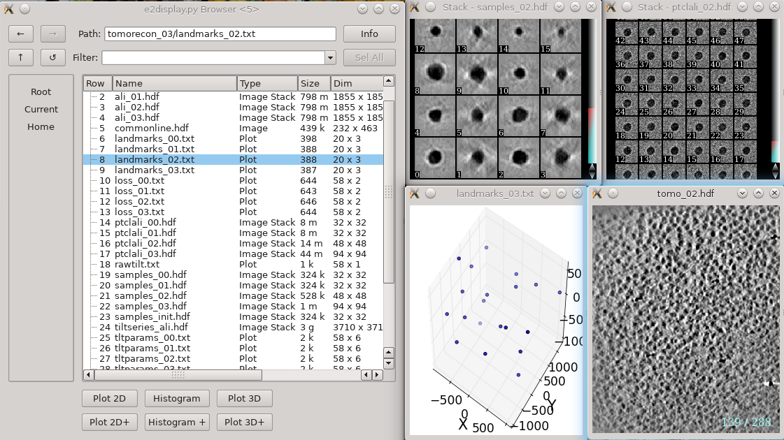
If you wish to look at the intermediate aligned tilt-series and other files, uncheck notmp, but note that this will significantly increase disk requirements
- This is not required for the remaining steps in the tutorial, but can be used to help understand how the tomogram alignment works. This requires significant additional disk space. You may consider doing this for only one tomogram.
In each tomorecon_XX folder
landmark_0X.txt has the location of the landmarks (which may be fiducials if present) in each iteration
samples_0X.hdf shows the top and side view of those landmarks
ptclali_0X.hdf has the trace of each landmark throughout the tilt series (they should stay at the center of image all the time if the alignment is good)
tomo_0X.hdf is the reconstruction after each iteration
- Launch
When working with your own data:
Either specify the correct tltstep if the tilt series is in order from one extreme to the other, or specify the name of a rawtlt file (as produced by serialem/IMOD).
While the program can automatically compute the orientation of the tilt axis, it can lead to a handedness ambiguity in the tomogram (it happens to be correct in the tutorial data). For your own data, it is recommended to confirm the handedness in a few good tomograms, then provide the correct tltax value for the reconstruction of all tomograms. To determine the handedness computationally, try the tutorial here for EMAN2 build after 05/23/2019 (or EMAN>=2.31).
In most cases, the default npk should be fine. If fiducials are present, it is not necessary to adjust this number to match the number of fiducials. The program will use any high contrast areas it finds as potential landmarks.
bytile should normally be selected, as it will normally produce better quality reconstructions at higher speed. If 2k or larger tomograms are created, memory consumption may be high, and you should check the program output for the anticipated RAM usage.
- The graphical interface only permits 1k or 2k reconstruction sizes. In our experience this is normally sufficient for segmentation or particle picking.
When the sample is thick, some grid-like tiling pattern can be seen in the reconstruction. Checking extrapad can largely reduce the artifacts. In versions after 2/3/2020, there is also a moretile option that further eliminates them. Note these artifacts will NOT impact the subtomogram averaging results because the particles are extracted in a separate process. Checking these options can make the reconstruction process more memory consuming, and up to 5 times slower.
When the sample is thin (purified protein, not cells), it is useful to check correctrot to automatically position tomograms flat in ice
It can also be helpful with thin ice to specify a clipz value to generate thinner tomograms (perhaps 64 or 96 for a 1k tomogram).
Handedness Check (can be skipped in the tutorial)
EMAN2 includes a novel procedure for determining the correct tilt axis for a tilt series based on defocus estimates across the tilted images in a tilt series. The tutorial data set comes out correctly without running this check, but when working with your own data, this step is highly recommended. Once you know the correct tilt axis direction to use for a given microscope/camera, you shouldn't need to run this test on every data set, but it may not be a bad idea even then, as there are various possible configuration/software errors on the instrument which could potentially cause inconsistent results.
For the tutorial tilt-series:
Subtomogram Averaging -> CTF Estimation
tiltseries = select any one tilt series
alltiltseries = not selected
voltage and cs (double check that values are correct)
checkhand = selected
- Launch
You will need to look at the console where you launched e2projectmanager to see the results of the test. It should look something like:
Average score: Current hand - 4.133, flipped hand - 3.290
Defocus std: Current hand - 0.110, flipped hand - 0.165
Current hand is better than the flipped hand in 86.4% tilt images
The handedness (--tltax=-4.1) seems to be correct. Rerun CTF estimation without the checkhand option to finish the process.
If you run this check on multiple images and it seems that they indicate a tilt axis/handedness error, then you need to return to the previous step (Tomogram Reconstruction) and run this again for all of your tomograms, with the correct tilt axis entered in the corresponding box. The same tilt axis should be used for all tilt series collected under the same conditions on the same instrument.
Note: This method removes almost all of the ambiguity about particle handedness. The one potential issue is that the MRC file format uses a non-conventional origin for images. If the data collection software doesn't take this into account, the images may be flipped when written to disk. The easiest way to check the software would be to collect 2 images of the same target and save them directly into different file formats, then checking (in different software) whether the two images appear to have the same handedness
CTF Estimation (<10 min)
For the tutorial tilt-series:
Subtomogram Averaging -> CTF Estimation
alltiltseries = selected, note that doing this will override anything present in the tiltseries field
checkhand = not selected
- Launch
When working with your own data:
The first two options, dfrange and psrange indicate the defocus and phase shift range to search. They take the format of “start, end, step”, so “2, 5, .1” will search defocus from 2 to 5 um with a step size of 0.1. Units for phase shift is degrees.
For images taken with volta phase plate, we usually have dfrange of “0.2,2,0.1” and psrange of “60,120,2”.
Note: this program is only estimating CTF parameters, taking tilt into account. It is not performing any phase-flipping corrections on whole tomograms. CTF correction is performed later as a per-particle process. This process requires metadata determined during tilt-series alignment, so it cannot be used with tomograms reconstructed using other software packages.
Note: In >2022 snapshots of EMAN2 it is possible after CTF correction to return to the 3-D reconstruction step and produce CTF corrected whole tomograms, but this does nothing useful when following the EMAN2 pipeline. If you wish to compare EMAN2 tomograms with other software doing CTF correction, this could potentially be useful
Tomogram reconstruction evaluation (optional)
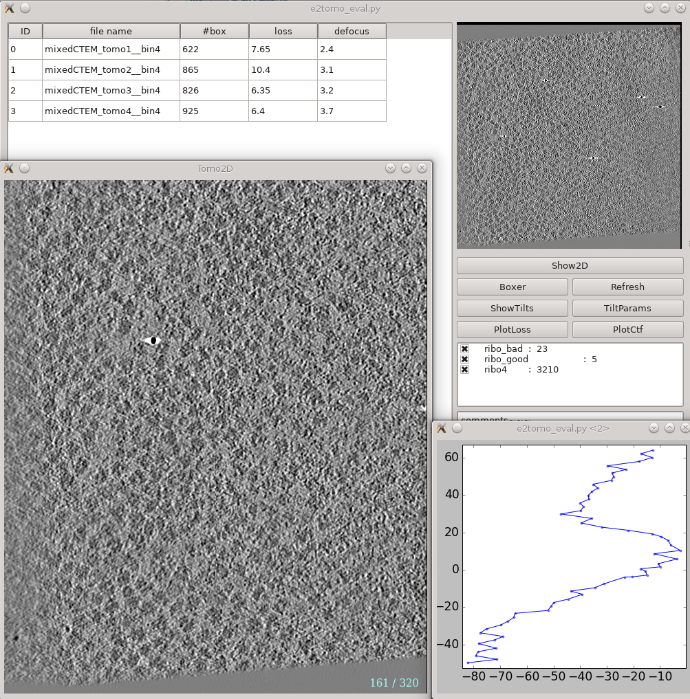
Analysis and visualization -> Evaluate tomograms can be used to evaluate the quality of your tilt series alignments and tomogram reconstructions. This tool will show more information as you progress through the tutorial, but can be used already at this point to make various assessments of your tomograms. Note that some of this information may not be available if you had notmp checked during the reconstruction.
- On the left is a list of tomograms in the project.
- Clicking the header of any column will sort the table by that attribute.
#box is the number of boxes in the tomogram
loss is the average landmark uncertainty in nm. You should not try to compare this number to, for example, the fiducial alignment error in IMOD, as it is computed in a completely different way. This number can be useful to identify specific tilt series within a project which aren't aligning as well as others, but the absolute number is not a useful value to report/analyze. Even if this number were >5 nm, it is still quite possible to achieve a subnanometer resolution subtomogram average.
defocus is the average defocus of the tilt series.
- On the right
- The image at the top is the central slice through the tomogram
the show2d button displays the selected tomogram in a slice-wise view.
ShowTilts shows the corresponding raw tilt series
- Please note that most tomograms include some out-of-plane tilt (the actual rotation isn't a simple tilt along a single axis), which is taken into account during alignment. This may make it visually appear that the tilt series alignment is not as robust as it actually is.
Boxer opens the 3D particle picker
PlotLoss will plot the fiducial error for each tilt
PlotCtf plot the defocus and phase shift at the center of each tilt image
Tiltparams is a bit more complicated. It plots a point list with 6 columns and a number of rows corresponding to the images in the selected tilt series. These are the alignment parameters for the tilt series.
You can adjust X Col and Y Col in the plot control panel (middle click the plot). The columns represent:
- 0 - tilt ID
- 1 - translation along x
- 2 - translation along y
- 3 - tilt angle around y
- 4 - tilt angle around x
- 5 - tilt angle around z
- The first panel below the buttons are the types of particles and how many of that type are in the project
- The last box is reserved for comments for each tomogram. You can fill in any comments you have on a specific tomogram and it will be saved for future reference.
Tomogram annotation (optional alternative to process below, GPU recommended)
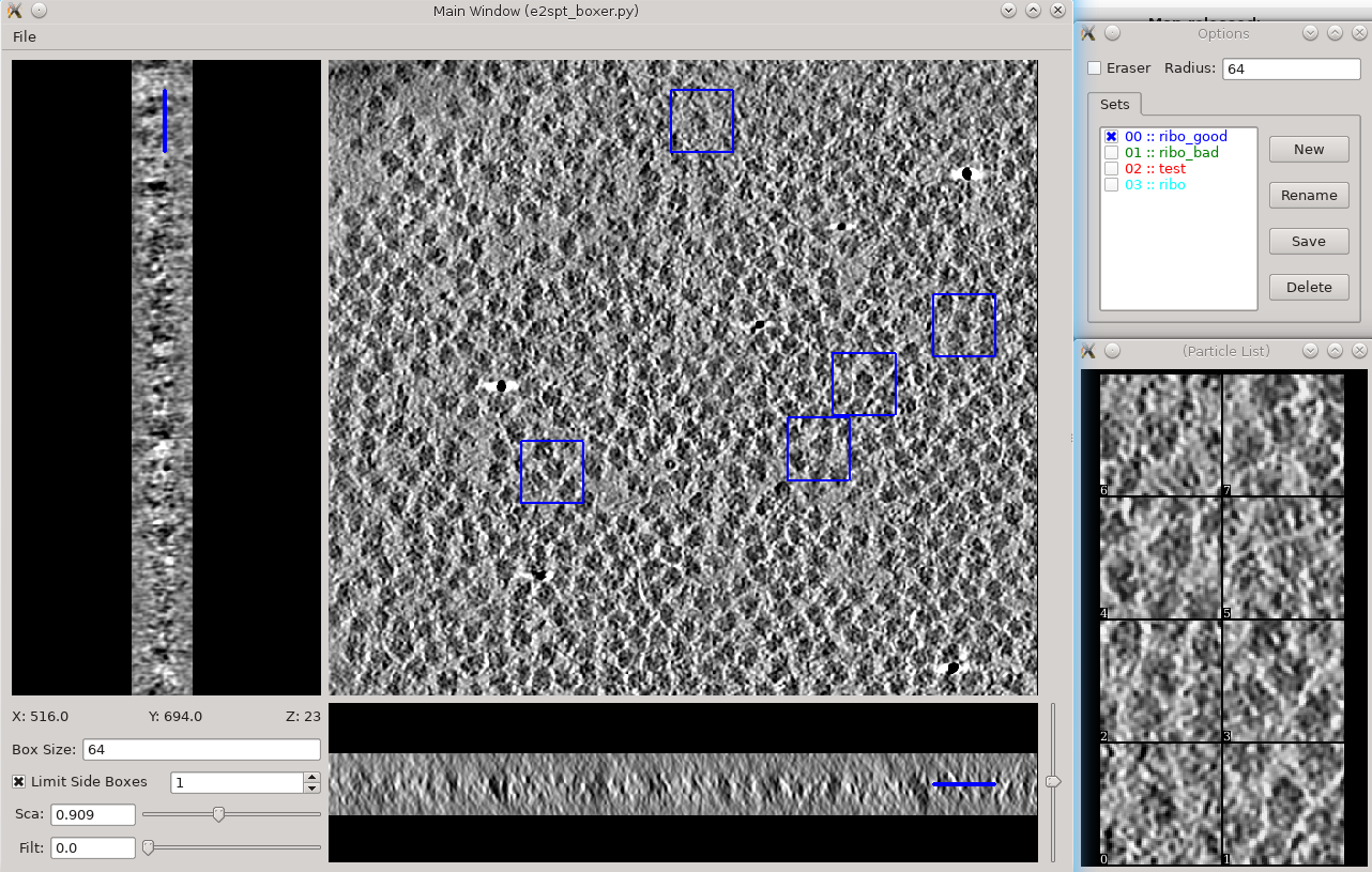
- Since the tutorial data set is purified ribosomes, this step can be skipped for the tutorial data, and you can move on to template-based particle picking. For cells or other types of complex specimens, tomogram annotation can be used to produce locations of different types of objects.
There is a newer tool which can be used for deep-learning based particle picking, which is really a different task than annotation. If you have a GPU and prefer this over the reference based approach outlined in the next section, see: New automatic particle picking. The annotation tool is still functional and available, but is targeted more at annotation of cellular features: TomoSeg
This is a brief summary of the annotation-based approach:
Segmentation -> Preprocess tomogram
- This step is not always necessary for tomograms reconstructed in EMAN2, but may slightly improve results.
Segmentation -> Box Training References
- This is a newer interface than previously used for this step. Select a few "Good" (regions containing the feature of interest) and "Bad" (regions not containing the feature of interest) boxes.
- "~" and "1" on the keyboard can be used to move along the Z axis.
- The new interface permits different types of features to be identified in a single session and in the same tomogram.
If the different features of interest have very different scale, it is always better to keep the box size at 64, and instead rescale the tomogram. As long as the rescaling is done using EMAN2 utilities, the program will correctly keep track of the geometry relative to the original tomogram & tilt series.
- if you are doing this with the tutorial data, you would only have 2 classes of particles "ribo_good" and "ribo_bad".
When pressing Save all visible particles (box checked next to the class name) will be saved
The rest of the annotation process remain unchanged from the original tutorial, except that now, all trained neural networks and training results are saved in the neuralnets folder, and all segmented maps are in the segmentations folder. You now only specify the label of the output file instead of the full file name.
Segmentation -> Find particles from segmentation to turn segmented maps into particle coordinates.
- Input both the tomogram and its corresponding segmentation, and the particles coordinates will be written into the metadata file.
- Slightly tweaking the threshold parameters may yield better results.
featurename will become the label of particles generated. Those particles can be viewed in the particle picking step and processed in the following protocols.
Particle picking (10-15 min)
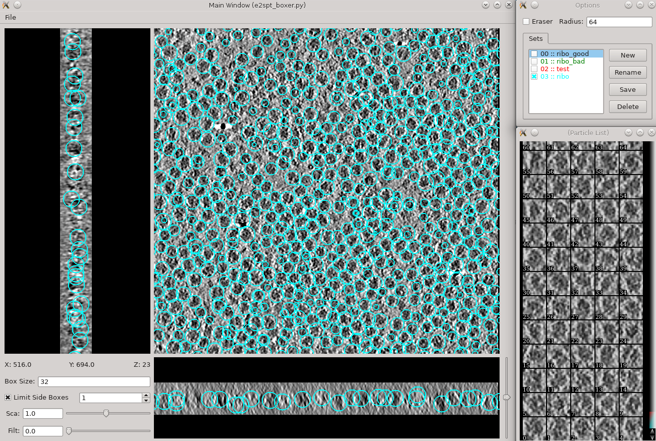
- Time above is to manually select 30-50 reference particles.
- You can launch the particle picker in two equivalent ways:
Subtomogram averaging -> Manual boxing, select tomogram, Launch
Analysis and visualization -> Evaluate tomograms as above, press the "Boxer" button
two windows will appear Main Window and Options. If you don't see Options it is probably hiding behind the main window.
in the Options window, rename the set of boxes to "initribo". This will be used as the label in later stages
- The box size can be set in the main window at the left bottom corner, for this tutorial, use 32 for ribosomes (the unbinned box size is 128).
This is NOT the same as the size listed near the word erase in another window, which is the size of the eraser.
- left click and drag to place and reposition boxes in any of the 3 views
- Hold down Shift when clicking to delete existing boxes.
- Boxes are shown as circles, which vary in size depending on the Z distance from the center of the particle.
- If you accidentally include one or more particles with nearby gold fiducials or other high contrast artifacts, it may cause some issues with your generated model (do not do that).
Go through slices along z-axis using ‘~’ and ‘1’ on the keyboard, or using the slider in the lower right of the window
It may be easier to locate particles if you adjust the Filt slider to ~70, but it will slow things down
- The interface supports different box types within a single tomogram. Each type has a label. Make sure the label is consistent if selecting the same feature in different tomograms.
- If you skipped the tomogram annotation step, we will pick a few particles here to generate an initial model, and use the initial model as a reference for template matching.
- Select 30-50 particles from one tomogram, then close the boxer window.
Do not use the Save button in the Options window or any of the menu items related to saving data. Those are available for special purposes. When you change the boxes, your changes are saved immediately and automatically. When you are done, simply close the main window.
- If you did the previous optional annotation step above, you will be able to see the selected particles here, and if you like, manually update them.
Particle extraction (2 min)
In this pipeline, the full 1k or 2k tomograms are used only as a reference to identify the location of the objects to be averaged. Now that we have particle locations, the software returns to the original tilt-series, extracts a per-particle tilt-series, and reconstructs each particle in 3-D independently.
For the tutorial tilt-series:
Subtomogram Averaging -> Extract Particles
check alltomograms
set boxsz_unbin to 128.
- If you had the correct size in the previous step this should be the same as leaving the default -1
- It is fine to use a different (usually larger) box size here if you find it easier to select particles with a smaller box size. For the tutorial, stick with 128, though.
- enter the label you used when picking particles ("initribo" if you followed the instructions above)
threads = value for your machine
- Launch
Subtomogram Averaging -> Build Sets
check allparticles
- Launch
- This will generate particle sets, which are virtual particle stacks that consist of particles with the same label from different tomograms.
For your own data
If the box size is correct when you select particles from the GUI, you can leave boxsz_unbin as -1, so the program will keep that box size (scaled to the original tilt series)
If your particles are deeply buried in other densities, using a bigger padtwod may help, but doing so may significantly increase the memory usage and slow down the process.
With CTF information present, it generally does not hurt to check wiener, which filters the 2D particles by SSNR before reconstructing them in 3D.
Specify a binning factor in shrink to produce downsampled particles if your memory/storage/CPU time is limited, but it will also limit the resolution you can achieve.
Initial model generation (10 - 60 min)
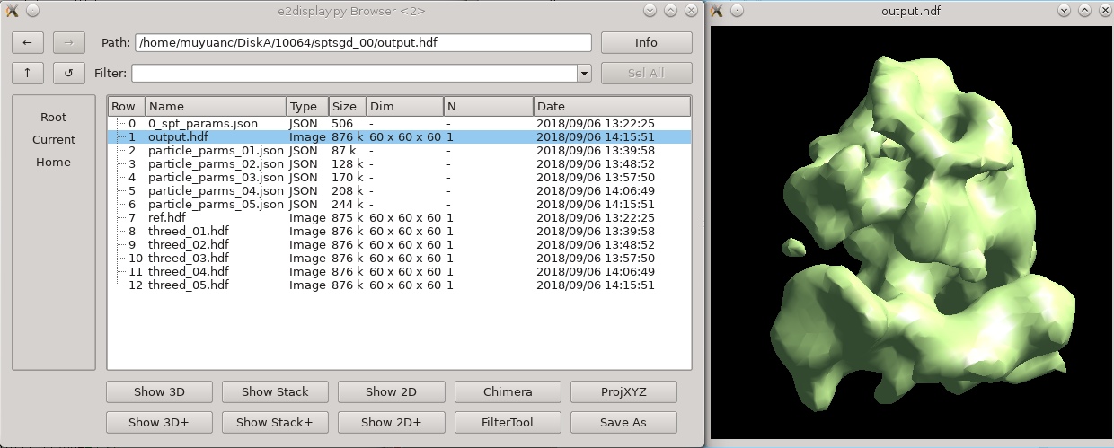
While intuitively it seems like (since the particles are already in 3-D) the concept of an "initial model" should not be necessary. Unfortunately, due to the missing wedge, and the low resolution of one individual particle (particularly from cells), it is actually critical to make a good starting average. Historically it has been challenging to get a good starting model, depending on the shape of the molecule. This new procedure based on stochastic gradient descent has proven to be quite robust, but it is difficult for the computer to tell when it has converged sufficiently. For this reason, the default behavior is to run much longer than is normally required, and have a human decide when it's "good enough" and terminate the process. If you use a small shrink value and let it run to completion, it can take some time to run. This is harmless, but unnecessary.
For the tutorial tilt-series:
Subtomogram Averaging -> Generate Initial Model
particles should be set to the sets/initribo.lst file you just created (or whatever name you used).
set shrink to 2, 3 or 4
- 2 will run slowly but will produce a more detailed initial model (not really necessary)
increasing batchsize will use more cores (if you have more than 12), and may cause it to converge to the correct answer in fewer iterations, but each iteration will not become faster.
The default niter of 5 is typically much more than is required
- Launch
You can terminate the job as soon as sptsgd_00/output.hdf looks reasonable. If you display the progress monitor (4th icon on the right side of the project manager), you can easily kill the job when you're happy. Usually this will take about 10 minutes for the tutorial data.
For your own data:
If your particle has known symmetry, specify that EMAN2/Symmetry
The symmetry you specify will not be imposed on the map unless you also check applysym, but the map will be rotationally aligned so the symmetry axes are in the correct direction, which will make it easier to apply symmetry in later steps. We do not generally recommend checking this box in this step.
setting shrink to something in the range of 2-4 will make the runtime faster but, depending on the shape, could potentially cause problems.
- using more than the minimal 30-50 particles is fine. If you have a very large set of selected particles, go ahead and use them all. This will not slow the process down at all, since it's stochastic.
it is critical that the full sampling box size of the extracted particles divided by shrink be divisible by 2. If not, the program will crash.
Template matching (5 min)
In this step, we will use the initial model you just produced as a template for finding all of the ribosomes in all 4 tomograms. If you completed the Tomogram Annotation step above, and have already extracted a full set of 1000+ particles, then you can skip this step, as we already have all of the particles. Note that here, and everywhere else in the tomography pipeline, reconstructed particles have positive contrast (look white in projection) and tomograms/tilt series have negative contrast (look dark in projection). If you wish to use a reference volume from the PDB or somesuch, then it should have positive contrast as is normal in the single particle CryoEM field.
Subtomogram Averaging -> Reference Based Boxing
browse to select tomograms. Select all 3 tomograms.
set reference to the output.hdf file you produced in the previous step.
set label to "ribo"
set nptcl to 150 (the maximum number of particles per tomogram)
IMPORTANT NOTE: There are more particles than this in these images. We limit this to 150 from each tomogram so the tutorial runs faster. If you are unconcerned with speed, you can increase this number, but if you're doing that, you may consider running the full tutorial instead.
- Launch
when this finishes, you can use the same Manual Boxing tool you used before to look at the particles which were selected. You may wish to manually remove any bad particles it selected. For the tutorial data set or other tomograms of purified protein, this process should work pretty well. For cells you might wish to use the Tomogram Annotation method above.
- note that this process stores 3-D particle locations in the appropriate info/* files, but does not extract particles from the micrographs
Particle extraction (~15 min)
Again, if you already did Tomogram Annotation above, this step isn't necessary. It is only required if you just did Template Matching.
Since this involves several thousand particles instead of 30-50, it will take quite a lot longer to run. The actual time will depend partially on the speed of your storage.
For the tutorial tilt-series:
Subtomogram Averaging -> Extract Particles
check alltomograms
set boxsz_unbin to 128.
set label to "ribo"
- Launch
Subtomogram Averaging -> Build Sets
check allparticles
- Launch
- This will generate particle sets, which are virtual particle stacks that consist of particles with the same label from different tomograms.
Subtomogram refinement (~1 hr/iteration)
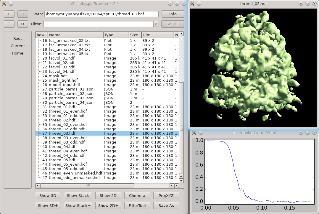
This step performs a conventional iterative subtomogram averaging using the full set of particles. Typically it will achieve resolutions in the 15-25 A range with a reasonable number of particles. As it involves 3-D alignment of the full set of particles multiple times, it takes a significant amount of compute time. Higher resolutions are achieved in the next stage after this (subtilt refinement).
For the tutorial tilt-series:
Subtomogram Averaging -> 3D Refinement
set particles to "sets/ribo.lst"
set reference to "output.hdf" from Initial Model Generation
set goldstandard to 30
set mass to 3000
set threads to the number of CPUs on your machine
- Launch
Results will gradually appear in spt_XX/ Feel free to look at intermediate results with the EMAN2 file browser as they appear.
For your own data:
- If your molecule has symmetry, you should specify it, but it's important that the alignment reference you provide has been properly aligned to the symmetry axes of whichever symmetry you specify.
localfilter will use e2fsc.py to compute a local resolution map after each iteration and filter the map accordingly. This is useful for molecules with significant variability.
If you suspect that a large fraction of your particles are "bad" in some way, you may wish to try reducing pkeep, which will hopefully exclude bad particles preferentially over "good" particles.
Subtilt refinement (~9 hr/iteration)
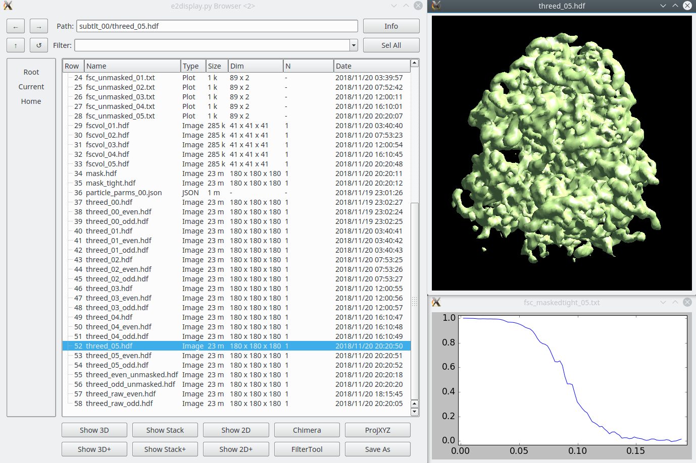
With the results of a good subtomogram alignment/average, we are now ready to switch to alignment of the individual particle images in each tilt, along with per-particle-per-tilt CTF correction and other refinements. This is effectively a hybrid of single particle analysis and subtomogram averaging, and can readily achieve subnanometer resolution IF the data is of sufficient quality. The tutorial data set is, but many cellular tomograms, for example, are not collected with high resolution in mind, and even with this sort of refinement will be unable to achieve resolutions better than 10-30 A, depending on the data. This process is completely automatic, based on all of the metadata collected up to this point. While it is possible to perform "subtomogram refinement" with subtomograms from any tomogram, Subtilt Refinement cannot operate properly unless all preceding steps occurred within EMAN2.
For the tutorial tilt series:
Subtomogram Averaging -> Sub-tilt Refinement
path should be set to the name of one of a "spt_XX" folder to use as a starting point for the refinement
iter can be -1 to use the last complete iteration in the "spt_XX" folder. Alternatively you can specify a specific iteration to use
parallel should be "thread:N" where N is the number of cores you wish to use on a single machine. This job can be run on a linux cluster if you like: EMAN2/Parallel.
threads should also be set to the number of cores to use on a single machine
- Launch
For your own data:
niters is the number of iterations to run. The default of 4 should achieve convergence in most cases.
keep is the fraction of tilt images to use in the final map. This defaults to 0.5, meaning the worst 1/2 of the tilts for each particle will be discarded. This permits tilts which contain, for example, projections of fiducials or other strong densities, or with large amounts of motion to be automatically excluded in the final reconstruction.
maxalt specifies the maximum tilt angle to include from each particle. Most tilt series are collected such that the small tilt angles will have the least radiation damage, and very often high tilts suffer from more motion artifacts. If you enter, for example, "45" in this box then tilts <-45 and >45 will be discarded automatically. In most cases keep will already serve a similar purpose.
Congratulations! The final result of the tutorial will be found in "subtlt_00/". The final 3-D map will be "threed_04.hdf" with the default parameters. The final gold standard resolution curve will be "fsc_maskedtight_04.txt". The optional steps below are tools you can use to evaluate your results in more detail.
Refinement evaluation (optional)
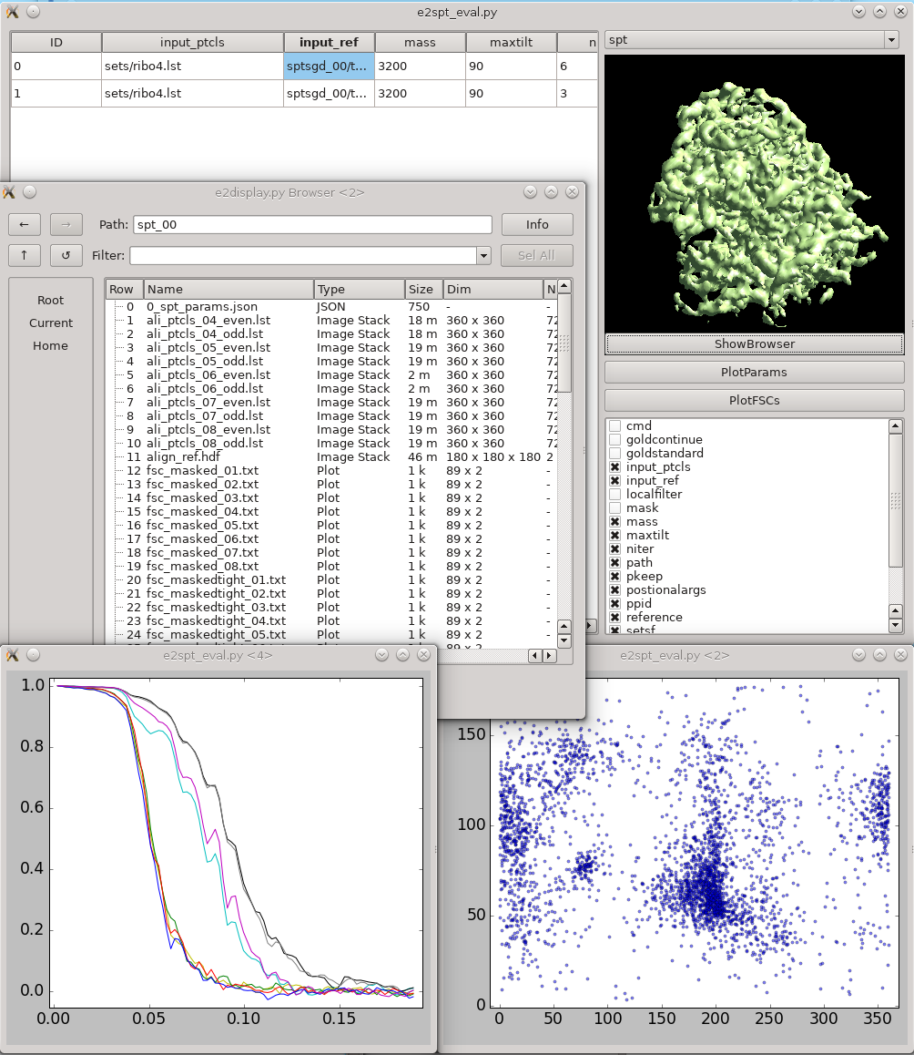 This tool helps visualize and compare results from multiple subtomogram refinement runs.
Analysis and Visualization -> Evaluate SPT Refinements
In the GUI, you can look at all spt_XX or sptsgd_XX folders and compare the parameters which were used for each, as well as the resulting maps.
- Switch between folder types using the menu at top right.
- Columns can be sorted by clicking on the corresponding header.
- Uncheck items in the list at bottom-right to hide corresponding columns
ShowBrowser will bring up the e2display.py browser in the folder of the selected row.
!PlotFSC will display the "tight" FSC curve over all iterations.
PlotParams will plot the Euler angle distribution and other alignment parameters
- The 8 columns in the plot are:
- 0 - az (EMAN convention Euler angle)
- 1 - alt
- 2 - phi
- 3 - translation in X
- 4 - Y
- 5 - Z
- 6 - alignment score
- 7 - missing wedge coverage
- The 8 columns in the plot are:
